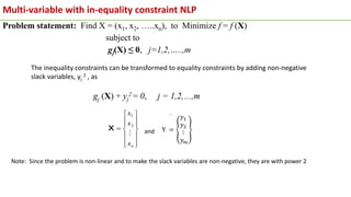
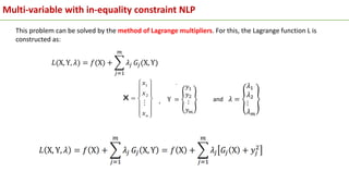
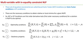
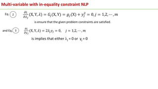
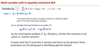
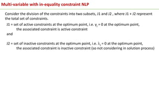
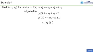
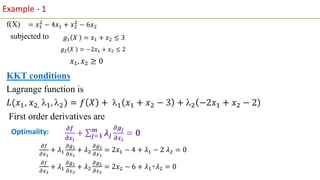
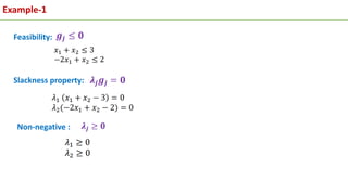
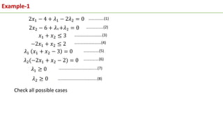
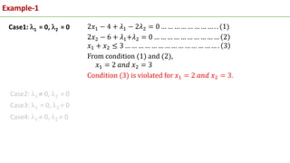
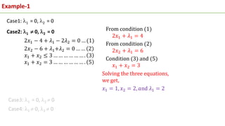
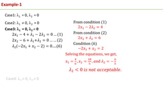
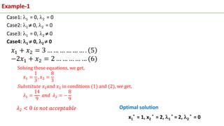
Multi-variable Optimization with in-equality constraints
Module-5: Classical Optimization Techniques
Multi-variable with in-equality constraint NLP
Problem statement: Find X = (x1, x2, …..xn), to Minimize f = f (X)
subject to
gj(X) ≤ 0, j=1,2,…..,m
The inequality constraints can be transformed to equality constraints by adding non-negative
slack variables, yj
2 , as
Note: Since the problem is non-linear and to make the slack variables are non-negative, they are with power 2















n
x
x
x

2
1
X and
Multi-variable with in-equality constraint NLP
This problem can be solved by the method of Lagrange multipliers. For this, the Lagrange function L is
constructed as:















n
x
x
x

2
1
X , and
Multi-variable with in-equality constraint NLP
The Lagrange function L is :
Necessary conditions:
1
2
3
System: No. of unknowns = n + 2 m, and No. of equations = n + 2 m
Solution: The solution gives the optimum solution vector X*, the Lagrange multiplier
vector, *, and the slack variable vector, Y*
Multi-variable with in-equality constraint NLP
• These set of equations (constraints) are called Karush Kuhn-Tucker (KKT) Conditions (or Kuhn-Tucker
conditions or KT conditions).
• These are the necessary conditions to obtain relative or local minima for a given NLPP.
• So, KKT or KT Conditions are first order derivative tests (first order necessary conditions) for a solution
in NLPP to be optimal.
1
2
3
Eq. - Optimality conditions
Eq. - Feasibility conditions
Eq. - Slackness property
Multi-variable with in-equality constraint NLP
2
Eq.
and Eq. 3
is ensure that the given problem constraints are satisfied.
is implies that either j = 0 or yj = 0
Multi-variable with in-equality constraint NLP
3
Consider Eq.
Case i : 𝝀𝒋 = 𝟎, then 𝒚𝒋 ≠ 𝟎.
This means that the given in-equality constraint is satisfied at given
point x* for local minimization problem.
Let us consider the local minima is at a point, X* :
So, for minimization problem, if 𝝀𝒋 = 𝟎 (and yj  0) then the constrain is not
active i.e. inactive constrain.
It means that the jth constraint is inactive and hence can be ignored. These
constraints are not taking part in identifying optimal solution.
Multi-variable with in-equality constraint NLP
3
Consider Eq.
Case ii : 𝝀𝒋  𝟎, then 𝒚𝒋 = 𝟎.
This means that the given in-equality constraint is becoming equality
constraint.
Let us consider the local minima is at a point, X* :
It means that the jth constraint is active and taking part in identifying optimal solution.
So, when 𝝀𝒋 ≠ 𝟎 (i.e. ) the associated constraint is active constraint and we
concentrate more on this case.
Multi-variable with in-equality constraint NLP
Consider the division of the constraints into two subsets, J1 and J2 , where J1 + J2 represent
the total set of constraints.
J1 = set of active constraints at the optimum point, i.e. yj = 0 at the optimum point,
the associated constraint is active constraint
and
J2 = set of inactive constraints at the optimum point, i.e. j = 0 at the optimum point,
the associated constraint is inactive constraint (so not considering in solution process)
Example-4
Darla
Find X(x1, x2) for minimize f(X)
subjected to
Example - 1
f(X)
subjected to
KKT conditions
Lagrange function is
𝐿(𝑥1, 𝑥2, 1, 2) = 𝑓 𝑋 + 1 𝑥1 + 𝑥2 − 3 + 2 −2𝑥1 + 𝑥2 − 2
First order derivatives are
Optimality:
Example-1
Non-negative :
Feasibility:
Slackness property:
Example-1
Check all possible cases
…………….(1)
………………(2)
…………….(5)
…………….(6)
………………………………....(7)
……………………………….….(8)
……………………….(4)
………………………..(3)
Example-1
Case1: 1 = 0, 2 = 0
Case2: 1  0, 2 = 0
Case3: 1 = 0, 2  0
Case4: 1  0, 2  0
Case1: 1 = 0, 2 = 0
Case2: 1  0, 2 = 0
Case3: 1 = 0, 2  0
Case4: 1  0, 2  0
Example-1
Example-1
Case1: 1 = 0, 2 = 0
Case2: 1  0, 2 = 0
Case3: 1 = 0, 2  0
Case4: 1  0, 2  0
Example-1
Case1: 1 = 0, 2 = 0
Case2: 1  0, 2 = 0
Case3: 1 = 0, 2  0
Case4: 1  0, 2  0
Optimal solution
x1
* = 1, x2
* = 2, 1
* = 2, 2
* = 0

5 Kuhn-Tucker Conditions explained for optimization

  • 1.
    Multi-variable Optimization within-equality constraints Module-5: Classical Optimization Techniques
  • 2.
    Multi-variable with in-equalityconstraint NLP Problem statement: Find X = (x1, x2, …..xn), to Minimize f = f (X) subject to gj(X) ≤ 0, j=1,2,…..,m The inequality constraints can be transformed to equality constraints by adding non-negative slack variables, yj 2 , as Note: Since the problem is non-linear and to make the slack variables are non-negative, they are with power 2                n x x x  2 1 X and
  • 3.
    Multi-variable with in-equalityconstraint NLP This problem can be solved by the method of Lagrange multipliers. For this, the Lagrange function L is constructed as:                n x x x  2 1 X , and
  • 4.
    Multi-variable with in-equalityconstraint NLP The Lagrange function L is : Necessary conditions: 1 2 3 System: No. of unknowns = n + 2 m, and No. of equations = n + 2 m Solution: The solution gives the optimum solution vector X*, the Lagrange multiplier vector, *, and the slack variable vector, Y*
  • 5.
    Multi-variable with in-equalityconstraint NLP • These set of equations (constraints) are called Karush Kuhn-Tucker (KKT) Conditions (or Kuhn-Tucker conditions or KT conditions). • These are the necessary conditions to obtain relative or local minima for a given NLPP. • So, KKT or KT Conditions are first order derivative tests (first order necessary conditions) for a solution in NLPP to be optimal. 1 2 3 Eq. - Optimality conditions Eq. - Feasibility conditions Eq. - Slackness property
  • 6.
    Multi-variable with in-equalityconstraint NLP 2 Eq. and Eq. 3 is ensure that the given problem constraints are satisfied. is implies that either j = 0 or yj = 0
  • 7.
    Multi-variable with in-equalityconstraint NLP 3 Consider Eq. Case i : 𝝀𝒋 = 𝟎, then 𝒚𝒋 ≠ 𝟎. This means that the given in-equality constraint is satisfied at given point x* for local minimization problem. Let us consider the local minima is at a point, X* : So, for minimization problem, if 𝝀𝒋 = 𝟎 (and yj  0) then the constrain is not active i.e. inactive constrain. It means that the jth constraint is inactive and hence can be ignored. These constraints are not taking part in identifying optimal solution.
  • 8.
    Multi-variable with in-equalityconstraint NLP 3 Consider Eq. Case ii : 𝝀𝒋  𝟎, then 𝒚𝒋 = 𝟎. This means that the given in-equality constraint is becoming equality constraint. Let us consider the local minima is at a point, X* : It means that the jth constraint is active and taking part in identifying optimal solution. So, when 𝝀𝒋 ≠ 𝟎 (i.e. ) the associated constraint is active constraint and we concentrate more on this case.
  • 9.
    Multi-variable with in-equalityconstraint NLP Consider the division of the constraints into two subsets, J1 and J2 , where J1 + J2 represent the total set of constraints. J1 = set of active constraints at the optimum point, i.e. yj = 0 at the optimum point, the associated constraint is active constraint and J2 = set of inactive constraints at the optimum point, i.e. j = 0 at the optimum point, the associated constraint is inactive constraint (so not considering in solution process)
  • 10.
    Example-4 Darla Find X(x1, x2)for minimize f(X) subjected to
  • 11.
    Example - 1 f(X) subjectedto KKT conditions Lagrange function is 𝐿(𝑥1, 𝑥2, 1, 2) = 𝑓 𝑋 + 1 𝑥1 + 𝑥2 − 3 + 2 −2𝑥1 + 𝑥2 − 2 First order derivatives are Optimality:
  • 12.
  • 13.
    Example-1 Check all possiblecases …………….(1) ………………(2) …………….(5) …………….(6) ………………………………....(7) ……………………………….….(8) ……………………….(4) ………………………..(3)
  • 14.
    Example-1 Case1: 1 =0, 2 = 0 Case2: 1  0, 2 = 0 Case3: 1 = 0, 2  0 Case4: 1  0, 2  0
  • 15.
    Case1: 1 =0, 2 = 0 Case2: 1  0, 2 = 0 Case3: 1 = 0, 2  0 Case4: 1  0, 2  0 Example-1
  • 16.
    Example-1 Case1: 1 =0, 2 = 0 Case2: 1  0, 2 = 0 Case3: 1 = 0, 2  0 Case4: 1  0, 2  0
  • 17.
    Example-1 Case1: 1 =0, 2 = 0 Case2: 1  0, 2 = 0 Case3: 1 = 0, 2  0 Case4: 1  0, 2  0 Optimal solution x1 * = 1, x2 * = 2, 1 * = 2, 2 * = 0