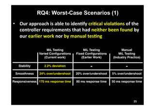
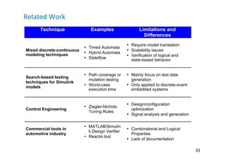
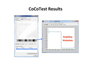
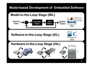
This document describes research on model-in-the-loop (MiL) testing of highly configurable continuous controllers. The researchers developed an approach using dimensionality reduction, surrogate modeling, and search-based techniques to efficiently test controllers across large configuration spaces. They applied their approach to an industrial conveyor belt controller case study. Evaluation results showed that their technique could find stability, smoothness, and responsiveness violations that previous approaches had missed. It provided a scalable way to thoroughly test continuous controller models over varied parameter configurations.

1. MiL Testing of
Highly Configurable Continuous Controllers:
Scalable Search Using Surrogate Models
Reza Matinnejad
Shiva Nejati
Lionel Briand
Software Verification and Validation Group
SnT Center, University of Luxembourg
Thomas Bruckmann
Delphi Automotive Systems, Luxembourg

2. Closed-loop Continuous Controllers
An Example: Conveyor Belt Controller
Controller
1

3. Closed-loop Continuous Controllers
An Example: Conveyor Belt Controller
+
-­‐
2
Closed-loop
Controller

4. Closed-loop Continuous Controllers
3

5. Model-based Development of Embedded Software
Model-in-the-Loop Stage (MiL)
Desired
Value
Controller
Model
System
Output
Plant
Model
+
-
Hardware-in-the-Loop Stage (HiL)
4
Software-in-the-Loop Stage (SiL)

6. MiL Testing Continuous Controllers (1)
Configuration 1
Configuration 2
Configuration 3
Controller
Model
Plant
Model
5
Instantiating the Controller Model
• Step1: Identifying an assignment of values to the
configuration parameters of the controller model

7. MiL Testing Continuous Controllers (2)
• Step2: Running simulations of the controller model
and examining the output signals
Desired/Actual Value
Running Model Simulation
Desired/Actual Value
Time Time
6
Test Input 1
/ Output 1 Test Input 2 / Output 2

8. Controller Requirements (1)
• Stability: The actual value shall stabilize at the desired
value Actual Value
Time Time
Actual Value
7
Stability
Violation
Stability
Violation

9. Controller Requirements (2)
• Smoothness: The actual value shall not abruptly
change when it is close to the desired value
Time
Actual Value
8
Smoothness
Violation

10. Controller Requirements (2)
• Responsiveness: The controller shall respond within a
certain time-limit
9
Time
Actual Value
Responsiveness
Violation

11. Stability Objective Function: Fst
• Fst (Test Case A) > Fst (Test Case B)
• We look for test input that maximizes Fst
Test Case A Test Case B
Actual Value
Actual Value
Time Time
10

12. Smoothness Objective Function: Fsm
• Fsm (Test Case A) > Fsm (Test Case B)
• We look for test input that maximizes Fsm
Test Case A Test Case B
Actual Value Time Time
11
Actual Value

13. Responsiveness Objective Function: Fr
• Fr (Test Case A) > Fr (Test Case B)
• We look for test input that maximizes Fr
Actual Value
Test Case A Test Case B
Actual Value
Time Time
12

14. Our Approach:
Search-based Testing of Continuous Controllers
13
• Step 1 : Exploration
Controller-
Plant Model
• Step 2 : Search
Controller
Behavior
Over the
Input Space
1.Exploration
Plant ⌃
Controller
Worst-Case
Scenarios
Critical
Operating
Regions of
the Controller
2.Search

15. Our Earlier Work:
Search-based Testing of Continuous Controllers
with fixed values for the configuration parameters
1.Exploration 2.Single-state
ID FD
FD
ID
Smoothness HeatMap
Initial Desired (ID)
Final Desired (FD)
Smoothness Worst-case Scenario
Controller-plant
model
HeatMap
Diagram
Worst-Case
Scenarios
List of
Critical
Regions
Domain
Expert
search
Controller Input Space
Fst
Fsm
Fr
14
Published
in
[IST
Journal
2014,
SSBSE
2013]

16. 1. The input space of the controller is larger
• 6 configuration parameters in our case study
2. Not all the configuration parameters matter for
4. Search becomes slower
• It takes 30 sec to run each model Simulation
Controller-plant
model
Challenges When Searching
the Entire Configuration Space
1.Exploration 2.Single-state
HeatMap
Diagram
Worst-Case
Scenarios
List of
Critical
Regions
Domain
Expert
search
all the objective functions
3. Harder to visualize the results
15

17. Our approach for Testing the Controller
in the Entire Configuration Space
Dimensionality
ReducLon
to
focus
the
exploraLon
on
the
variables
with
significant
impact
on
each
objecLve
funcLon
Surrogate
Modeling
to
avoid
running
simulaLons
for
parts
of
the
input
space
where
the
surrogate
model
is
the
most
accurate.
VisualizaLon
of
the
8-­‐dimension
space
using
Regression
Trees
16
Controller-plant
model
+
Configuration
parameters
ranges
Regression
Trees
Worst-Case
Scenarios
List of
Critical
Regions
Domain
Expert
1.Exploration with
Dimensionality
Reduction
x<0.2
y<0.3
z<0.1
2. Search with
Surrogate
Modeling

18. Exploration with Dimensionality Reduction
Elementary Effects Analysis Method
• Goal:
IdenLfying
variables
with
a
significant
impact
on
each
objecLve
funcLon
17
Exploring
all the
dimensions
Exploring the
significant
dimensions
ProportionalGain
DerivativeGain
IntegralGain
IntgrResetErrLim
...
Smoothness
ProportionalGain
IntgrResetErrLim
...
Elementary
Effects
Analysis
Method
...

19. Regression Tree
• Goal:
Dividing
the
input
space
into
homogenous
parLLons
with
respect
to
the
objecLve
funcLon
values
Smoothness Regression Tree
18
All Points
ID < 0.7757
Count
Mean
Std Dev
Count
Mean
Std Dev
ID >= 0.7757
Count
Mean
Std Dev
FD >= 0.5674 FD < 0.5674
Count
Count
Mean
Mean
Std Dev
Std Dev
1000
0.007
0.0049
574
0.0059
0.004
426
0.0103425
0.0049919
182
0.0134
0.005
244
0.008
0.003
FD < 0.1254 FD >= 0.1254
Count
Mean
Std Dev
Count
Mean
Std Dev
182
0.0134555
0.0052883
244
0.0080206
0.0031751
Smoothness HeatMap
FD<0.5674
FD>=0.1254

20. Search With Surrogate Modeling
Supervised Machine Learning
• Goal:
To
predict
the
values
of
the
objecLve
funcLons
within
a
criLcal
parLLon
and
speed
up
the
search
Smoothness
Critical Partition
19
• Surrogate model predicts Fsm
with a given confidence level
A
B
• During the search, surrogate model
predicts Fsm for the next point:
1. Not confident about Fsm(B) and
Fsm(A) relation
• Run the simulation as before
2. Confident that Fsm(B) > Fsm(A)
• Run the simulation as before
3. Confident that Fsm(B) < Fsm(A)
• Avoid running the Simulation

21. Search With Surrogate Modeling
Supervised Machine Learning
• Different
Machine
Learning
techniques:
1. Linear
Regression
2. ExponenLal
Regression
3. Polynomial
Regression
(n=2)
4. Polynomial
Regression
(n=3)
• Criteria
to
compare
different
techniques:
1. R2
ranges
from
0
to
1
• R2
shows
goodness
of
fit
2. Mean
RelaLve
PredicLon
Error
(MRPE)
• MRPE
shows
predicLon
accuracy
20

22. Evaluation: Research Questions
• RQ1 (Which ML Technique): Which Machine Learning
technique performed the best?
21
• RQ2 (Effect of DR): What was the effect of
Dimensionality Reduction?
• RQ3 (SM vs. No-SM): How
did
the
search
with
Surrogate
Modeling
perform
comparing
to
the
search
without
Surrogate
Modeling?
• RQ4 (Worst-Case Scenarios): How
did
our
approach
perform
in
finding
worst-­‐case
test
scenarios?

23. RQ1: Which Machine Learning Technique?
22
• The
best
technique
to
build
surrogate
models
for
all
our
three
objecLve
funcLons
is
Polynomial
Regression
(n=3)
• PR
(n=3)
has
the
highest
R2
(
goodness
of
fit
)
• PR
(n=3)
has
the
smallest
MRPE
(
predicLon
error
)
• The
surrogate
models
are
accurate
and
predicLve
enough
for
Smoothness
and
Responsiveness
(R2
was
close
to
1,
MRPE
was
close
to
0)
• In
future,
we
want
to
try
other
Supervised
Leaning
techniques,
such
as
SVM

24. RQ2: Effect of Dimensionality Reduction
23
• Dimensionality
reducLon
helps
generate
beber
surrogate
models
for
Smoothness
and
Responsiveness
• Smaller
MRPE:
More
predicLve
surrogate
model
Smoothness Responsiveness
0.03
MRPE
0.02
DR 0.01 No DR
0.04
0.03
0.02
MRPE
DR No DR
Mean Relative Prediction Error (MRPE)

25. RQ3: Search with vs. without Surrogate Modeling
24
• For
responsiveness,
the
search
with
SM
was
8
Lmes
faster
0.17
0.165
0.16
Highest value
of Fr
After 300 Sec
After 2500 Sec
• For
0.17
0.165
smoothness,
the
search
with
SM
was
much
more
effecLve
Highest value
of Fsm
After 800 Sec
After 2500 Sec
SM No SM
0.23
0.225
0.22
SM No SM
0.23
0.225
0.22
SM
No SM
SM
0.16
SM No SM
No SM

26. RQ4: Worst-Case Scenarios (1)
25
• Our
approach
is
able
to
idenLfy
criLcal
violaLons
of
the
controller
requirements
that
had
neither
been
found
by
our
earlier
work
nor
by
manual
tesLng
MiL Testing
Varied Configurations
(Current work)
MiL Testing
Fixed Configurations
(Earlier Work)
Manual
MiL Testing
(Industry Practice)
Stability
Smoothness
Responsiveness
2.2% deviation - -
24% over/undershoot
170 ms response time
20% over/undershoot
80 ms response time
5% over/undershoot
50 ms response time

27. RQ4: Worst-Case Scenarios (2)
26
• For
example,
for
the
industrial
controller
we
idenLfied
the
following
violaLon
of
the
Stability
requirement
within
the
given
ranges
for
the
calibraLon
variables
ID = 0.36
2.2 % Deviation
FD = 0.22
Flap Position
Time

28. 27
Conclusion

29. 28
MiL Testing of
Highly Configurable Continuous Controllers:
Scalable Search Using Surrogate Models
Reza Matinnejad
PhD Candidate
Software Verification and Validation Group
SnT Center, University of Luxembourg
Emails: reza.matinnejad@uni.lu
r.matinnejad@gmail.com

30. Alternative Heatmap
ü Our approach was implemented at Technical
University of Munich too
Responsiveness Stability

31. ExisLng
Tool
Support
for
TesLng
Simulink/Stateflow
Models
• None
of
the
exis,ng
tools
specifically
test
the
con,nuous
proper,es
of
Simulink
output
signals

32. Related
Work
Technique Examples Limitations and
Differences
Mixed discrete-continuous
modeling techniques
• Timed Automata
• Hybrid Automata
• Stateflow
• Require model translation
• Scalability issues
• Verification of logical and
state-based behavior
Search-based testing
techniques for Simulink
models
• Path coverage or
mutation testing
• Worst-case
execution time
• Mainly focus on test data
generation
• Only applied to discrete-event
embedded systems
Control Engineering • Ziegler-Nichols
Tuning Rules
• Design/configuration
optimization
• Signal analysis and generation
Commercial tools in
automotive industry
• MATLAB/Simulin
k Design Verifier
• Reactis tool
• Combinatorial and Logical
Properties
• Lack of documentation
31

33. CoCoTest
Results
Stability
Violation
32