Download as PDF, PPTX


![Arrays
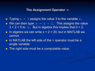
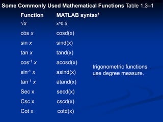
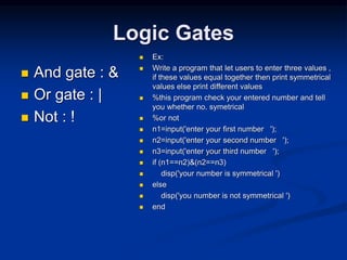
• The numbers 0, 0.1, 0.2, …, 10 can be assigned to the
variable u by typing u = [0:0.1:10].
• To compute w = 5 sin u for u = 0, 0.1, 0.2, …, 10, the
session is;
>>u = [0:0.1:10];
>>w = 5*sin(u);
• The single line, w = 5*sin(u), computed the formula
w = 5 sin u 101 times.](https://image.slidesharecdn.com/matlabch01-180829224953/85/Matlabch01-23-320.jpg)
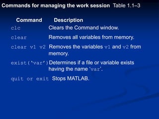
![Column Array
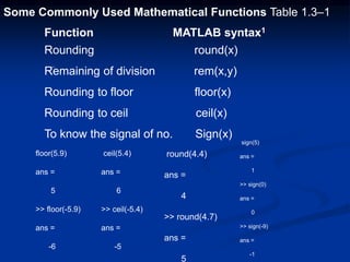
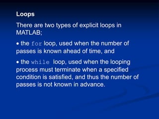
To make an array with one column and multi rows
use the following two modes
1- using semicolon x=[1;2;3;4;5;6;7;8;9;]
2- using single quote x=[1:9] ‘
Use length function to measure how many elements
are available in an array
Ex x=[1:9]';
>> length(x)
ans =
9](https://image.slidesharecdn.com/matlabch01-180829224953/85/Matlabch01-25-320.jpg)
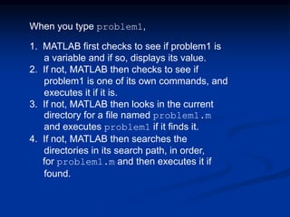
![Arrays Applications
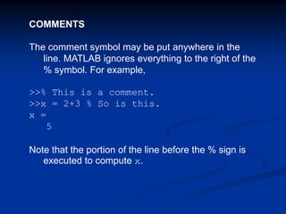
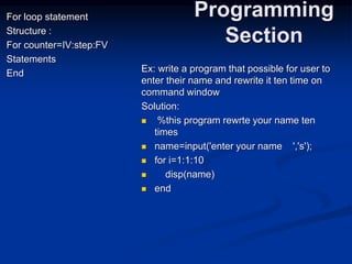
Summation & subtraction of arrays
Ex:
a1=[1:9]
a1 =
1 2 3 4 5 6 7 8 9
>> a2=[4:12]
a2 =
4 5 6 7 8 9 10 11 12
>> a1+a2
ans =
5 7 9 11 13 15 17 19 21
>> a1-a2
ans =
-3 -3 -3 -3 -3 -3 -3 -3 -3](https://image.slidesharecdn.com/matlabch01-180829224953/85/Matlabch01-26-320.jpg)
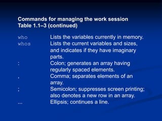
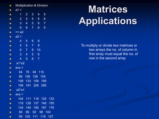
![Arrays Applications
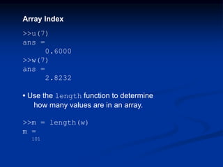
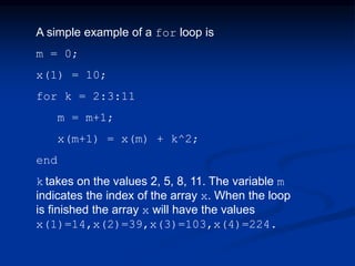
Multiplication and division
Ex:
a1=[1:9];
>> a2=[4:12]';
>> a1*a2
ans =
420
>> a2*a1
ans =
4 8 12 16 20 24 28 32 36
5 10 15 20 25 30 35 40 45
6 12 18 24 30 36 42 48 54
7 14 21 28 35 42 49 56 63
8 16 24 32 40 48 56 64 72
9 18 27 36 45 54 63 72 81
10 20 30 40 50 60 70 80 90
11 22 33 44 55 66 77 88 99
12 24 36 48 60 72 84 96 108
To multiply or divide two matrices or
two arrays the no. of column in
first array must equal the no. of
row in the second array](https://image.slidesharecdn.com/matlabch01-180829224953/85/Matlabch01-27-320.jpg)
![Arrays Applications
arrays construction methods
Ex:
a1=[1:3];
>> a2=[0.1:0.1:0.3];
>> a4=a1+a2
a4 =
1.1000 2.2000 3.3000
>> a3=[a1 a2]
a3 =
1.0000 2.0000 3.0000 0.1000 0.2000 0.3000](https://image.slidesharecdn.com/matlabch01-180829224953/85/Matlabch01-28-320.jpg)
![Arrays Applications
arrays construction methods
Ex:
a1=[1:3];
>> a2=[0.1:0.1:0.3];
>> a4=a1+a2
a4 =
1.1000 2.2000 3.3000
>> a3=[a1 ; a2]
a3 =
1.0000 2.0000 3.0000
0.1000 0.2000 0.3000](https://image.slidesharecdn.com/matlabch01-180829224953/85/Matlabch01-29-320.jpg)
![Arrays Applications
arrays elements change
Ex:
a2=[1:7];
a2(1,5)=9% or a(5)
a2 =
[ 1 2 3 4 9 6 7]
a3=[1:7]';
>> a3(4)=8 % or a3(4,1)=5
a3 =
1
2
3
8
5
6
7](https://image.slidesharecdn.com/matlabch01-180829224953/85/Matlabch01-30-320.jpg)
![Matrices Representation
To enter a matrix with m rows and n column
as follow
A= a11,a12,a13,…,a1n
: : : :
: : : :
am1,am2,am3,…,amn
Matlab expression
A=[a11,a12,…,a1n;a21,a22,…,a2n;…;amn]
( )](https://image.slidesharecdn.com/matlabch01-180829224953/85/Matlabch01-31-320.jpg)
![Matrices Representation
3x4 matrix
a=[1 2 3 4;5 6 7 8;9 10 11 12]
a =
1 2 3 4
5 6 7 8
9 10 11 12
2x2 matrix
> a1=[2,3;4 6]
a1 =
2 3
4 6](https://image.slidesharecdn.com/matlabch01-180829224953/85/Matlabch01-32-320.jpg)
![Matrices Index
a=[1 2 3 4;5 6 7 8;9 10 11 12]
a =
1 2 3 4
5 6 7 8
9 10 11 12
>> a(2,3)
ans =
7
a(4,4)
??? Index exceeds matrix dimensions.
](https://image.slidesharecdn.com/matlabch01-180829224953/85/Matlabch01-33-320.jpg)
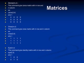
![Matrices
Applications
Adding and subtraction number
a1=[1:5;2:6;3:7]
a1 =
1 2 3 4 5
2 3 4 5 6
3 4 5 6 7
>> a1=a1+3
a1 =
4 5 6 7 8
5 6 7 8 9
6 7 8 9 10
Multiplication & division number
a1=a1/4
a1 =
1.0000 1.2500 1.5000 1.7500 2.0000
1.2500 1.5000 1.7500 2.0000 2.2500
1.5000 1.7500 2.0000 2.2500 2.5000](https://image.slidesharecdn.com/matlabch01-180829224953/85/Matlabch01-34-320.jpg)
![Matrices
Applications
Subtraction & Addition
a1=[1:5;2:6;3:7]
a1 =
1 2 3 4 5
2 3 4 5 6
3 4 5 6 7
>> a2=[4:8;5:9;6:10]
a2 =
4 5 6 7 8
5 6 7 8 9
6 7 8 9 10
>> a1-a2
ans =
-3 -3 -3 -3 -3
-3 -3 -3 -3 -3
-3 -3 -3 -3 -3
>> a1+a2
ans =
5 7 9 11 13
7 9 11 13 15
9 11 13 15 17](https://image.slidesharecdn.com/matlabch01-180829224953/85/Matlabch01-35-320.jpg)
![Matrices
Applications
Column Adding
a1 =
1 2 3 4 5
2 3 4 5 6
3 4 5 6 7
9 8 7 6 5
a1(:,5)=5 % or a1(1:end,5)=[5 5 5 5] or a1(1:4,5)=5
a1 =
1 2 3 4 5
2 3 4 5 5
3 4 5 6 5
9 8 7 6 5
Removing column
a1 =
1 2 3 4 5
2 3 4 5 5
3 4 5 6 5
9 8 7 6 5
a1(:,5)=[ ]
a1 =
1 2 3 4
2 3 4 5
3 4 5 6
9 8 7 6](https://image.slidesharecdn.com/matlabch01-180829224953/85/Matlabch01-37-320.jpg)
![Matrices
Applications
Row Adding
a1 =
1 2 3 4 5
2 3 4 5 6
3 4 5 6 7
9 8 7 6 5
a1(5,1:end)=5
a1 =
1 2 3 4
2 3 4 5
3 4 5 6
9 8 7 6
5 5 5 5
Removing row
a1 =
1 2 3 4
2 3 4 5
3 4 5 6
9 8 7 6
5 5 5 5
a1(5,:)=[ ]
a1 =
1 2 3 4
2 3 4 5
3 4 5 6
9 8 7 6](https://image.slidesharecdn.com/matlabch01-180829224953/85/Matlabch01-38-320.jpg)
![Matrices
Applications
Elements changing
a1 =
1 2 3 4
2 3 4 5
3 4 5 6
9 8 7 6
>> a1(3,3)=5
a1 =
1 2 3 4
2 3 4 5
3 4 5 6
9 8 7 6
a1(1:2,2:3)=[6 8; 9 8]
a1 =
1 6 8 4
2 9 8 5
3 4 5 6
9 8 7 6
a1(:,1)=1
a1 =
1 6 8 4
1 9 8 5
1 4 5 6
1 8 7 6](https://image.slidesharecdn.com/matlabch01-180829224953/85/Matlabch01-39-320.jpg)
![Matrices
Dot product of vectors
b1=[1:7]
b1 =
1 2 3 4 5 6 7
>> b2=[4:10]
b2 =
4 5 6 7 8 9 10
>> b1*b2'
ans =
224
>> dot(b1,b2) % or dot(b2,b1)
ans =
224
.* :this command multiply every elements in the first matrix with the opposite element in the
second matrix
Ex:
a1=[1 2 3;1 2 3];
>> a2=[4 5 6;6 7 8];
>> a1.*a2
ans =
4 10 18
6 14 24](https://image.slidesharecdn.com/matlabch01-180829224953/85/Matlabch01-43-320.jpg)
![Matrices
./ :
a1=[1 2 3;1 2 3];
>> a2=[4 5 6;6 7 8];
>> a1./a2
ans =
0.2500 0.4000 0.5000
0.1667 0.2857 0.3750
.^ :
a1=[1 2 3;1 2 3];
>> a1.^2
ans =
1 4 9
1 4 9
a1=[1 2 3;1 2 3;5 6 7];
logm(a1)
ans =
-11.2390 + 2.6969i 12.0991 - 0.6097i 0.5736 - 0.7747i
23.6246 - 0.4446i -22.7645 + 2.5319i 0.5736 - 0.7747i
-10.7608 - 1.1980i 12.8638 - 1.6426i 1.6248 + 1.0543i
>> expm(a1)
ans =
1.0e+004 *
0.9206 1.2622 1.6039
0.9205 1.2623 1.6039
2.4802 3.4007 4.3213](https://image.slidesharecdn.com/matlabch01-180829224953/85/Matlabch01-44-320.jpg)
![Matrices
And
Arrays
Size(matrix name)
:give matrix or array
size
Ex:
a1=[1:7];
>> a2=[1:7]';
>> a3=[1 2 3;4 5 6;6 7
8;3 4 5];
>> size(a1)
ans =
1 7
>> size(a2)
ans =
7 1
>> size(a3)
ans =
4 3
max(matrix name) :give
maximum element in every
column
Ex:
a1=[1:7];
>> a2=[1:7]';
>> a3=[1 2 3;4 5 6;6 7 8;3 4 5];
max(a1)
ans =
7
>> max(a2)
ans =
7
>> max(a3)
ans =
6 7 8
>> max(max(a3))
ans =
8](https://image.slidesharecdn.com/matlabch01-180829224953/85/Matlabch01-45-320.jpg)
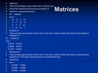
![Matrices
And
Arrays
length(matrix name)
:give matrix or array
length
Ex:
a1=[1:7];
>> a2=[1:7]';
>> a3=[1 2 3;4 5 6;6 7
8;3 4 5];
>> length(a1)
ans =
7
>> length(a2)
ans =
7
>> length(a3)
ans =
4
min(matrix name) :give
minimum element in every
column
Ex:
a1=[1:7];
>> a2=[1:7]';
>> a3=[1 2 3;4 5 6;6 7 8;3 4 5];
>> min(a1)
ans =
1
>> min(a2)
ans =
1
>> min(a3)
ans =
1 2 3
>> min(min(a3))
ans =
1](https://image.slidesharecdn.com/matlabch01-180829224953/85/Matlabch01-46-320.jpg)
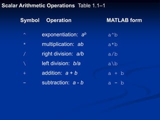
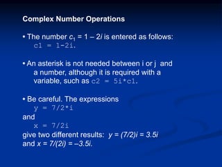
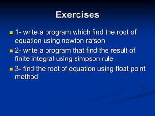
![Polynomial Roots
To find the roots of x3 – 7x2 + 40x – 34 = 0, the session
is
>>a = [1,-7,40,-34];
>>roots(a)
ans =
3.0000 + 5.000i
3.0000 - 5.000i
1.0000
The roots are x = 1 and x = 3 ± 5i.](https://image.slidesharecdn.com/matlabch01-180829224953/85/Matlabch01-47-320.jpg)
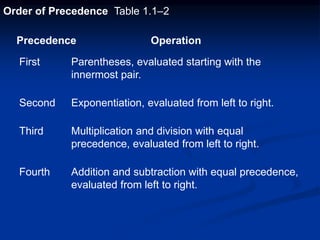
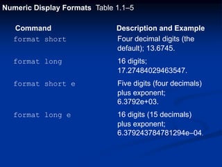
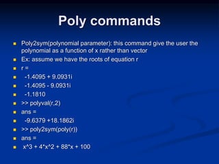
![Poly commands
Poly: This command opposite root command where this command
find the parameters of the polynomial if it’s roots has been found
Ex: x^3+4*x^2+88*x+100
r=[1 4 88 100]
r =
1 4 88 100
>> e=roots(r)
e =
-1.4095 + 9.0931i
-1.4095 - 9.0931i
-1.1810
>> poly(e)
ans =
1.0000 4.0000 88.0000 100.0000](https://image.slidesharecdn.com/matlabch01-180829224953/85/Matlabch01-48-320.jpg)
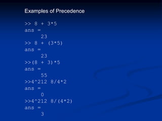
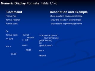
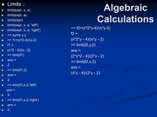
![Poly commands
Polyval(p,point): this command find the value of the polynomial at
specific point value
Where p : parameters of equation
Ex: x^3+4*x^2+88*x+100
p=[1 4 88 100]
p =
1 4 88 100
>> polyval(p,2)
ans =
300
polyval(r,[2 9 8])
ans =
300 1945 1572](https://image.slidesharecdn.com/matlabch01-180829224953/85/Matlabch01-49-320.jpg)
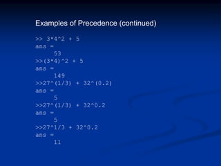
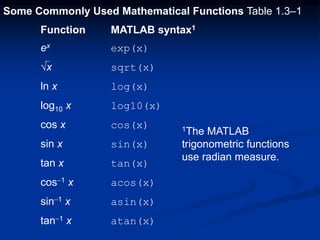
![Data
processing
Standard deviation :
Std(vector)
Ex:
a1 =
1 2 3 4 5 6 7
std(a1)
ans =
2.1602
Mean :
mean(a1)
ans =
4
Union:
a1=[1:7];
>> a2=[3:9];
>> union(a1,a2)
ans =
1 2 3 4 5 6
7 8 9
Intersection :
>> a1=[1:7];
>> a2=[3:9];
>> intersect(a1,a2)
ans =
3 4 5 6 7
Ismember :
ismember(9,a1)
ans =
0
>> ismember(2,a1)
ans =
1
Setdiff :
setdiff(a1,a2)
ans =
1 2
>> setdiff(a2,a1)
ans =
8 9](https://image.slidesharecdn.com/matlabch01-180829224953/85/Matlabch01-51-320.jpg)
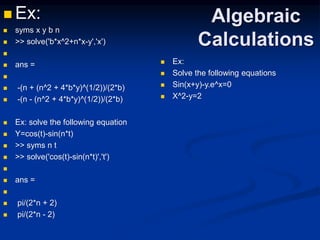
![Algebraic
Calculations
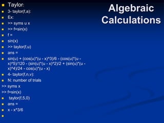
Syms : this command
used to declare a new
variable
Solve
(exp1,exp2…,expn,x1,x2,…,xn) :
Ex:
syms x
>> solve('x^2+3*x+2')
ans =
-2
-1
Ex:
>> syms x y
>> p=solve('x+5=0','y^3+y^2+y+1=0')
p =
x: [3x1 sym]
y: [3x1 sym]
>> p.x
ans =
-5
-5
-5
>> p.y
ans =
-1
i
-i](https://image.slidesharecdn.com/matlabch01-180829224953/85/Matlabch01-52-320.jpg)
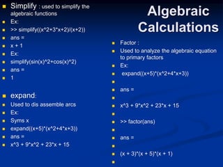
![Algebraic
Calculations
Root locus:
rlocus(sys)
rlocus(sys1,sys2,…,sysn)
Where f: transfer function
Ex:
h=tf([3 4 5],[3 4 5 6])
Transfer function:
3 s^2 + 4 s + 5
-----------------------
3 s^3 + 4 s^2 + 5 s + 6
>> rlocus(h)](https://image.slidesharecdn.com/matlabch01-180829224953/85/Matlabch01-59-320.jpg)
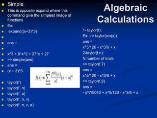
![Algebraic
Calculations
Nyquist criteria :
Nyquist(sys)
Nyquist(sys1,sys2,…,sysn)
Ex:
h=tf([3 4 5],[3 4 5 6])
Transfer function:
3 s^2 + 4 s + 5
-----------------------
3 s^3 + 4 s^2 + 5 s + 6
>> nyquist(h)](https://image.slidesharecdn.com/matlabch01-180829224953/85/Matlabch01-60-320.jpg)
![Algebraic
Calculations
Frequency response:
bode(sys)
bode(sys1,sys2,…,sysn)
Ex:
h=tf([3 4 5],[3 4 5 6])
Transfer function:
3 s^2 + 4 s + 5
-----------------------
3 s^3 + 4 s^2 + 5 s + 6
>> bode(h)](https://image.slidesharecdn.com/matlabch01-180829224953/85/Matlabch01-61-320.jpg)
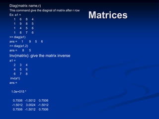
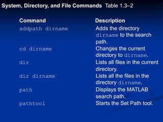
![Solution of Linear Algebraic Equations
6x + 12y + 4z = 70
7x – 2y + 3z = 5
2x + 8y – 9z = 64
>>A = [6,12,4;7,-2,3;2,8,-9];
>>B = [70;5;64];
>>Solution = AB
Solution =
3
5
-2
The solution is x = 3, y = 5, and z = –2.](https://image.slidesharecdn.com/matlabch01-180829224953/85/Matlabch01-62-320.jpg)
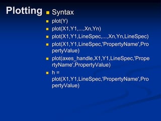
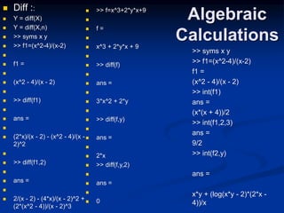
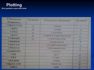
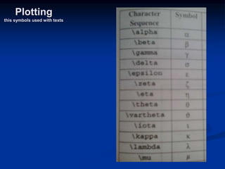
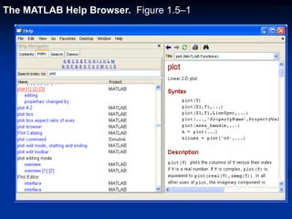
![Plotting
1- plot(Y)
Ex:
>> x=[1:10];
>> y=[10:-1:1];
>> plot(y)
>> plot(x,y)](https://image.slidesharecdn.com/matlabch01-180829224953/85/Matlabch01-64-320.jpg)
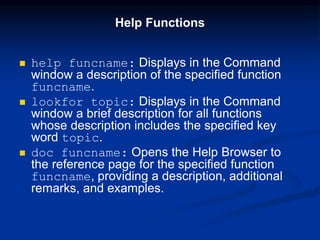
![Plotting
2- axis's name :
Xlabel
Ylabel
Title
Ex:
>> x=[1:10];
>> y=[10:-1:1];
>> plot(y)
>> plot(x,y) >> ylabel('torque')
>> xlabel('speed')
>> title('torque speed char.')](https://image.slidesharecdn.com/matlabch01-180829224953/85/Matlabch01-65-320.jpg)
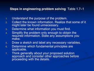
![Plotting
2- plot(x1,y1,…,xn,yn):
Ex:
>> x=[1:10];
>> y=sin(x);
>> w=[10:10:100];
>> z=cos(w);
>> plot(x,y,w,z)](https://image.slidesharecdn.com/matlabch01-180829224953/85/Matlabch01-66-320.jpg)
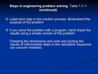
![Plotting
3- plot(X1,Y1,color of
Line(spec),...,Xn,Yn,colorof Line(Spec))
Ex:
>> x=[12:22];
>> y=[-12:-1:-22];
>> q=sin(x);
>> w=sin(y);
>> plot(x,q,'b',y,w,'m')
G: green
B:blue
K:black
W:white
M:pink
Y:yellow
R:red](https://image.slidesharecdn.com/matlabch01-180829224953/85/Matlabch01-67-320.jpg)
![Plotting
3- plot(X1,Y1,shape of
points(spec),...,Xn,Yn,shape of
points(Spec))
Ex:
>> x=[12:22];
>> y=[-12:-1:-22];
>> q=sin(x);
>> w=sin(y);
>> plot(x,q,'b',y,w,'m')
Some shapes you can use them
X, P , > ,< ,O , V , .
, * , H , SR .](https://image.slidesharecdn.com/matlabch01-180829224953/85/Matlabch01-68-320.jpg)
![Plotting
4- plot(X1,Y1,shape of points & line
(spec),...,Xn,Yn,shape of points & line
(Spec))
Ex:
>> x=[12:22];
>> y=[-12:-1:-22];
>> q=sin(x);
>> w=sin(y);
>> plot(x,q,'--SR',y,w,'-.*')
Some shapes you can use them
- , -.](https://image.slidesharecdn.com/matlabch01-180829224953/85/Matlabch01-69-320.jpg)
![Plotting
5- plot(X1,Y1,shape &color of points &
line (spec),...,Xn,Yn,shape & color of
points & line (Spec))
Ex:
>> x=[12:22];
>> y=[-12:-1:-22];
>> q=sin(x);
>> w=sin(y);
>> plot(x,q,'*r-.')](https://image.slidesharecdn.com/matlabch01-180829224953/85/Matlabch01-70-320.jpg)
![Plotting
6- figure : the aim of this command is to
plot multi functions in different figures not
on the same figure
Ex:
>> x=[12:22];
>> y=[-12:-1:-22];
>> q=sin(x);
>> w=sin(y);
>> plot(x,q,'*r-.')
>> figure
>> plot(y,w,'pg-.')](https://image.slidesharecdn.com/matlabch01-180829224953/85/Matlabch01-71-320.jpg)
![Plotting
7- subplot(m,n,p):
The aim of this command is plot a lot
of functions on the same figure without
overlapping
M: number of rows
N:number of columns
P: number of subplot
Ex:
>> x=[12:22];
>> y=[-12:-1:-22];
>> q=sin(x);
>> w=sin(y);
>> subplot(2,2,2)
>> plot(y,w,'pg-.')
>> subplot(2,2,3)
>> plot(x,q,'*r-.')](https://image.slidesharecdn.com/matlabch01-180829224953/85/Matlabch01-72-320.jpg)
![Plotting
8- axis:
A- axis(‘auto’) : give auto range for x & y axis
B- axis(‘equal’): the range of x and y is equal
together
C- axis(‘square’) :give square borders but not
same range
D-axis(‘off’): hide axis
Ex:
>> x=[12:22];
>> y=[-12:-1:-22];
>> q=sin(x);
>> w=sin(y);
>> plot(x,q,'*r-.')
>> axis('off')](https://image.slidesharecdn.com/matlabch01-180829224953/85/Matlabch01-73-320.jpg)
![Plotting
Ex:
>> x=[12:22];
>> y=[-12:-1:-22];
>> q=sin(x);
>> w=sin(y);
>> plot(x,q,'*r-.')
>> axis(on')
>> axis('square')](https://image.slidesharecdn.com/matlabch01-180829224953/85/Matlabch01-74-320.jpg)
![Plotting
Ex:
>> x=[12:22];
>> y=[-12:-1:-22];
>> q=sin(x);
>> w=sin(y);
>> plot(x,q,'*r-.')
>> axis(on')
>> axis(equal')](https://image.slidesharecdn.com/matlabch01-180829224953/85/Matlabch01-75-320.jpg)
![Plotting
9- grid:
Grid
Grid on
Grid off
This command divide the plot
figure into grids
>> x=[12:22];
>> y=[-12:-1:-22];
>> q=sin(x);
>> w=sin(y);
>> plot(x,q,'*r-.')
>> axis(on')
>> axis(equal')
>> grid on](https://image.slidesharecdn.com/matlabch01-180829224953/85/Matlabch01-76-320.jpg)
![Plotting
10- loglog:
loglog
Semilogx
Semilogy
This command convert the plot
axix from normal state into log
axis
>> x=[12:22];
>> y=1000*exp(x);
>> loglog(x,y)
>> axis(on')
>> grid on](https://image.slidesharecdn.com/matlabch01-180829224953/85/Matlabch01-77-320.jpg)
![Plotting
11- stem:
>> x=[12:22];
>> y=sin(x);
>> stem(x,y)](https://image.slidesharecdn.com/matlabch01-180829224953/85/Matlabch01-78-320.jpg)
![Plotting
11- stem:
>> x=[12:22];
>> y=sin(x);
>> stem(x,y,’pb-.’)](https://image.slidesharecdn.com/matlabch01-180829224953/85/Matlabch01-79-320.jpg)
![Plotting
12- hist:
>> x=[12:22];
>> y=sin(x);
>> stem(y)](https://image.slidesharecdn.com/matlabch01-180829224953/85/Matlabch01-80-320.jpg)
![Plotting
13- gtext(‘text’):
This command help user to write
any text in any place in figure
>> x=[12:22];
>> y=sin(x);
>> plot(x,y,'pb-.')
>> gtext('night of the light')](https://image.slidesharecdn.com/matlabch01-180829224953/85/Matlabch01-81-320.jpg)
![Plotting of
functions
14- ezplot:
ezplot(fun,[min,max])
ezplot(fun2)
ezplot(fun2,[xmin,xmax,ymin,ymax])
ezplot(fun2,[min,max])
ezplot(funx,funy)
ezplot(funx,funy,[tmin,tmax])
ezplot(...,figure_handle)
Ex:
>> syms x
>> ezplot('x^2-9')](https://image.slidesharecdn.com/matlabch01-180829224953/85/Matlabch01-84-320.jpg)
![Plotting of
functions
14- ezplot:
>> syms x
>> f=x^2-9
f =
x^2 - 9
>> ezplot(f,[-100 150])
Fun tool](https://image.slidesharecdn.com/matlabch01-180829224953/85/Matlabch01-85-320.jpg)


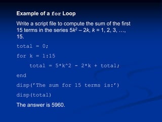
![Example of a Script File (continued)
% Calculation section:
dt = tf/500;
% Create an array of 501 time values.
t = [0:dt:tf];
% Compute speed values.
v = g*t;
%
% Output section:
Plot(t,v),xlabel(’t (s)’),ylabel(’v m/s)’)](https://image.slidesharecdn.com/matlabch01-180829224953/85/Matlabch01-97-320.jpg)
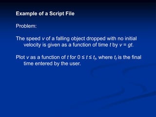
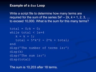
![Display(‘text’) or
disp(‘text’)
this command
used to display any
text on the
command window
You can use this
command in m-file
and command
window
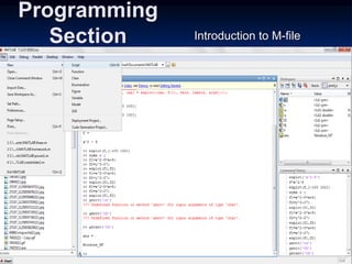
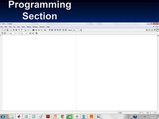
Programming
Section
>> disp('matlab')
matlab
>> x=[12:22];
>> display(x)
x =
12 13 14
15 16 17 18
19 20 21 22](https://image.slidesharecdn.com/matlabch01-180829224953/85/Matlabch01-98-320.jpg)
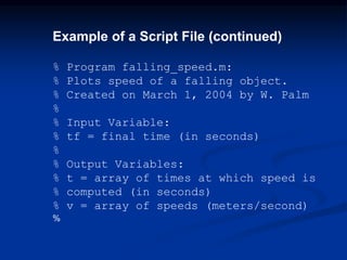
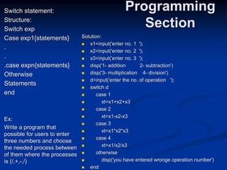
![input:
evalResponse = input(prompt)
strResponse = input(prompt, 's')
1- input(prompt):used to enter a number
from users
Ex:
>> r=input('enter number')
enter number7
r=
7
input(prompt, 's'): used to enter a string
from users
Ex:
>> str=input('enter your name ','s')
enter your name mohammad
str =
mohammad
Programming
Section Ex:
>> a=input('a=');
a=9
>> b=input('b=');
b=68
>> c=a+b;
>> disp(['c=',num2str(c)])
c=77
>> disp(sprintf('c=%d',c))
c=77](https://image.slidesharecdn.com/matlabch01-180829224953/85/Matlabch01-100-320.jpg)
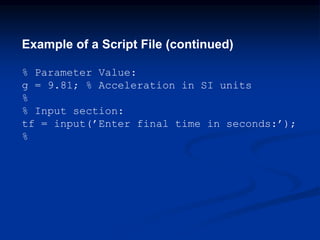
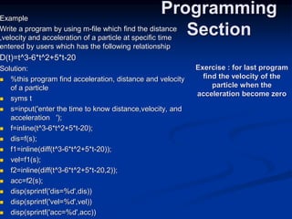
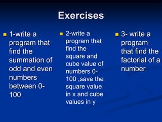
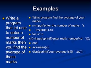
![Example
Write a program by using m-file which find the
area and circumference of a circle where users
enter the radius of circle.
Solution:
% this program find area and circumference of
a circle
r=input('enter the raduis of the circle ');
area=pi*r^2;
circumference=2*pi*r;
disp(sprintf('area=%f',area))
disp(sprintf('cicumference=%f',circumference))
u=[0:360];
x=r*cosd(u);
y=r*sind(u);
plot(x,y)
Programming
Section
Exercise : write a program
that find the area and
circumference of triangle](https://image.slidesharecdn.com/matlabch01-180829224953/85/Matlabch01-101-320.jpg)
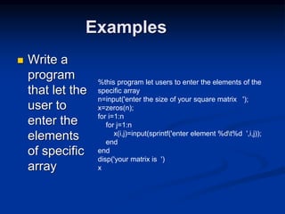
![Functions
Syntax
function [ output_args ] = Untitled( input_args )
End
The aim of functions is to design any function
which is not available in matlab or any function
belong any new subject](https://image.slidesharecdn.com/matlabch01-180829224953/85/Matlabch01-121-320.jpg)
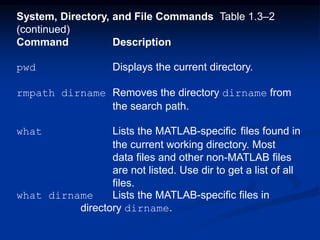

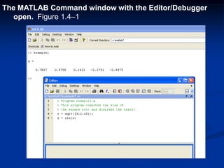
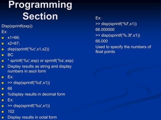
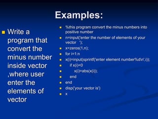
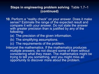
![The find Function
find(x) computes an array containing the indices of the
nonzero elements of the numeric array x. For example
>>x = [-2, 0, 4];
>>y = find(x)
Y =
1 3
The resulting array y = [1, 3] indicates that the first
and third elements of x are nonzero.](https://image.slidesharecdn.com/matlabch01-180829224953/85/Matlabch01-130-320.jpg)
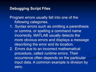
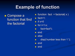
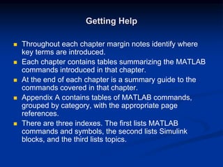
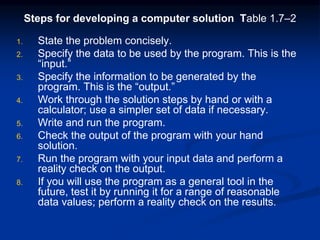
![Note the difference between the result obtained by
x(x<y) and the result obtained by find(x<y).
>>x = [6,3,9,11];y = [14,2,9,13];
>>values = x(x<y)
values =
6 11
>>how_many = length(values)
how_many =
2
>>indices = find(x<y)
indices =
1 4](https://image.slidesharecdn.com/matlabch01-180829224953/85/Matlabch01-131-320.jpg)

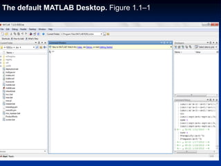
This document provides an overview of MATLAB including: 1. How to perform operations interactively or using script files 2. Entering commands and expressions using the command window 3. Examples of arithmetic, precedence rules, and assignment 4. Common mathematical functions and operations on arrays and matrices 5. Saving, loading, and managing variables and files in MATLAB sessions