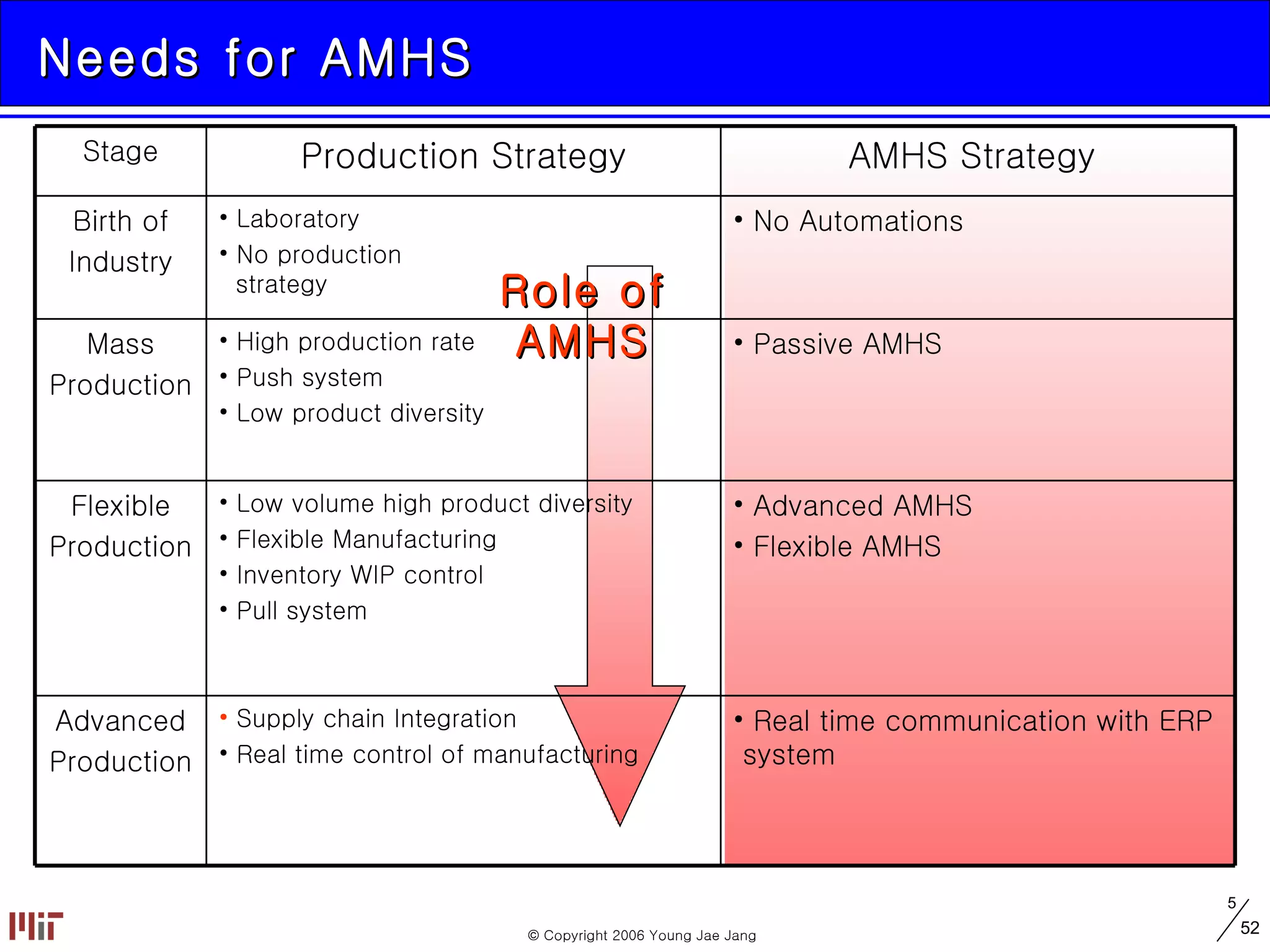
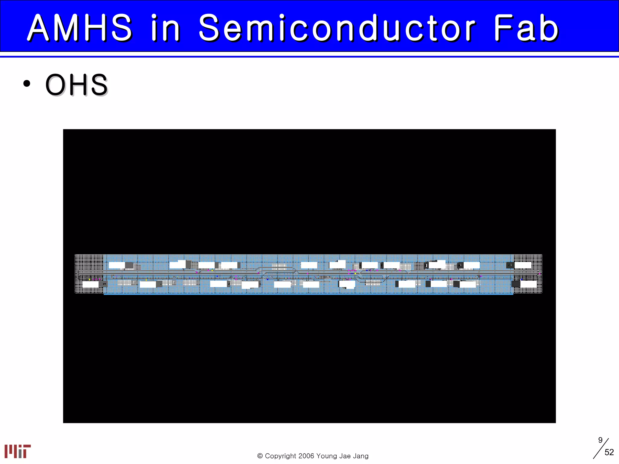
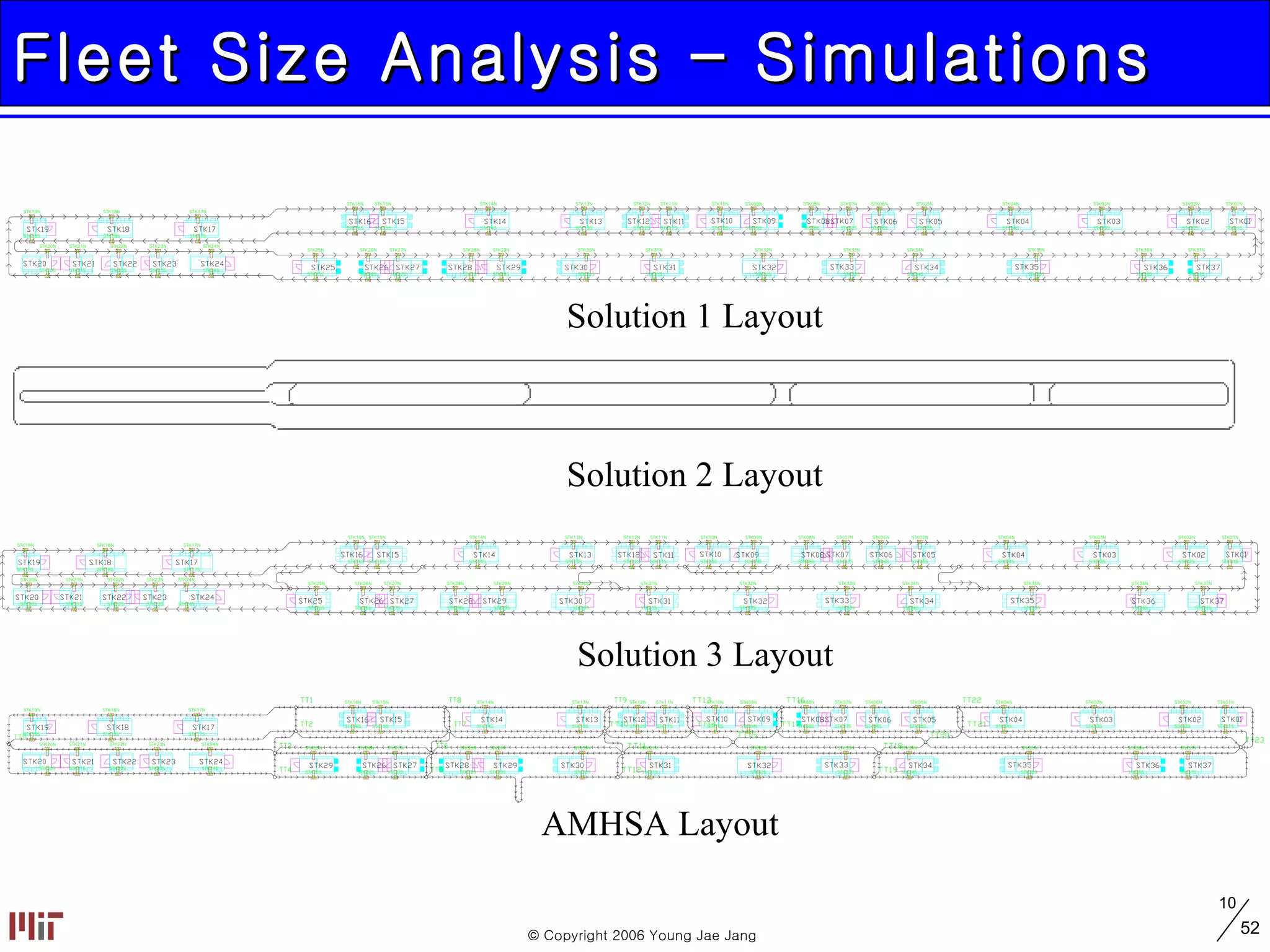
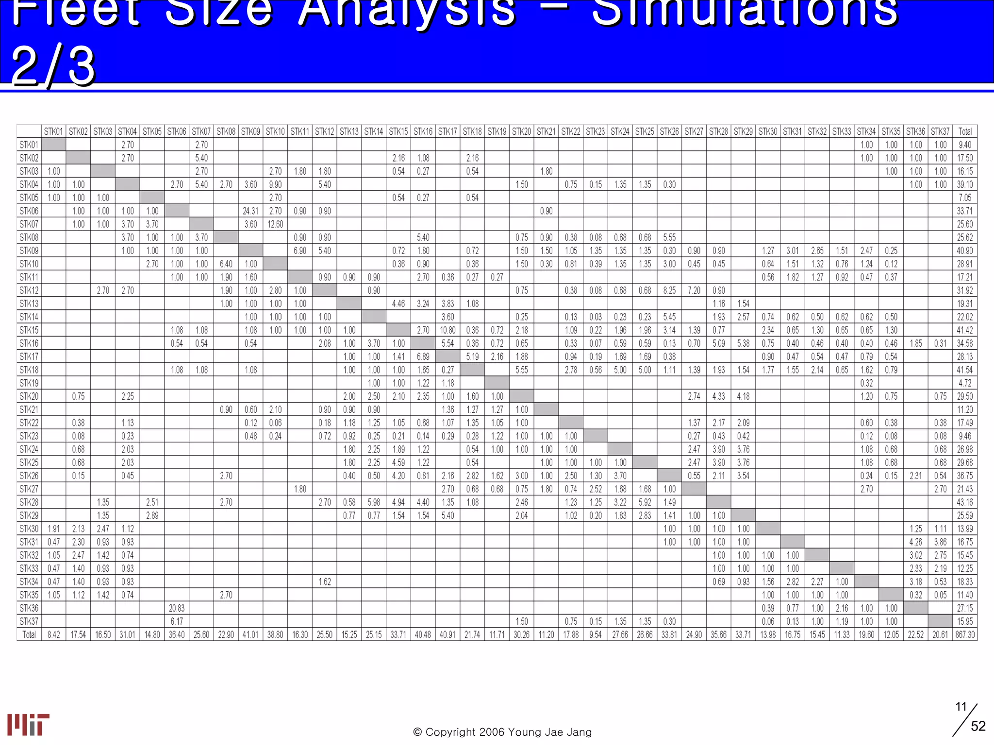
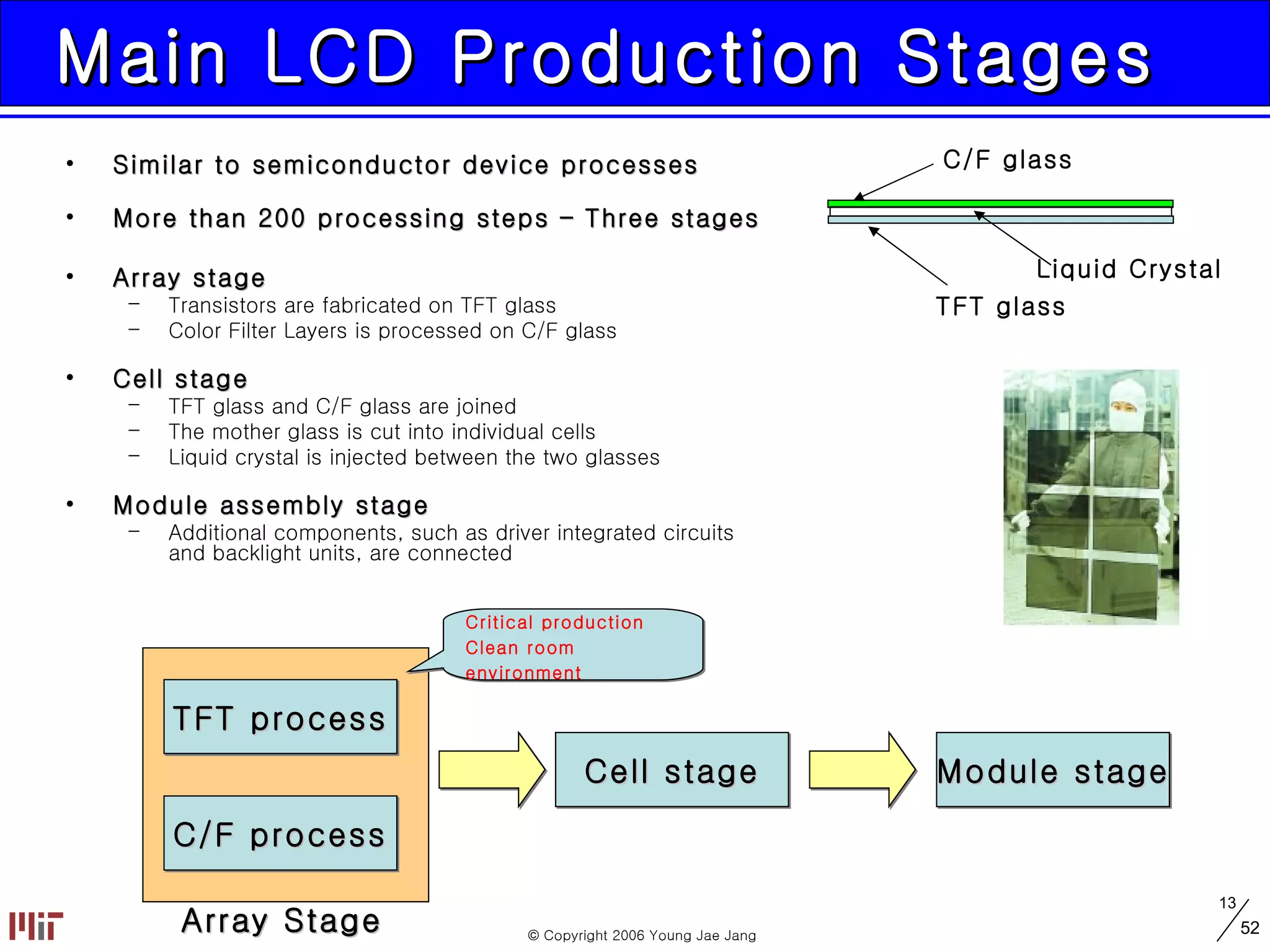
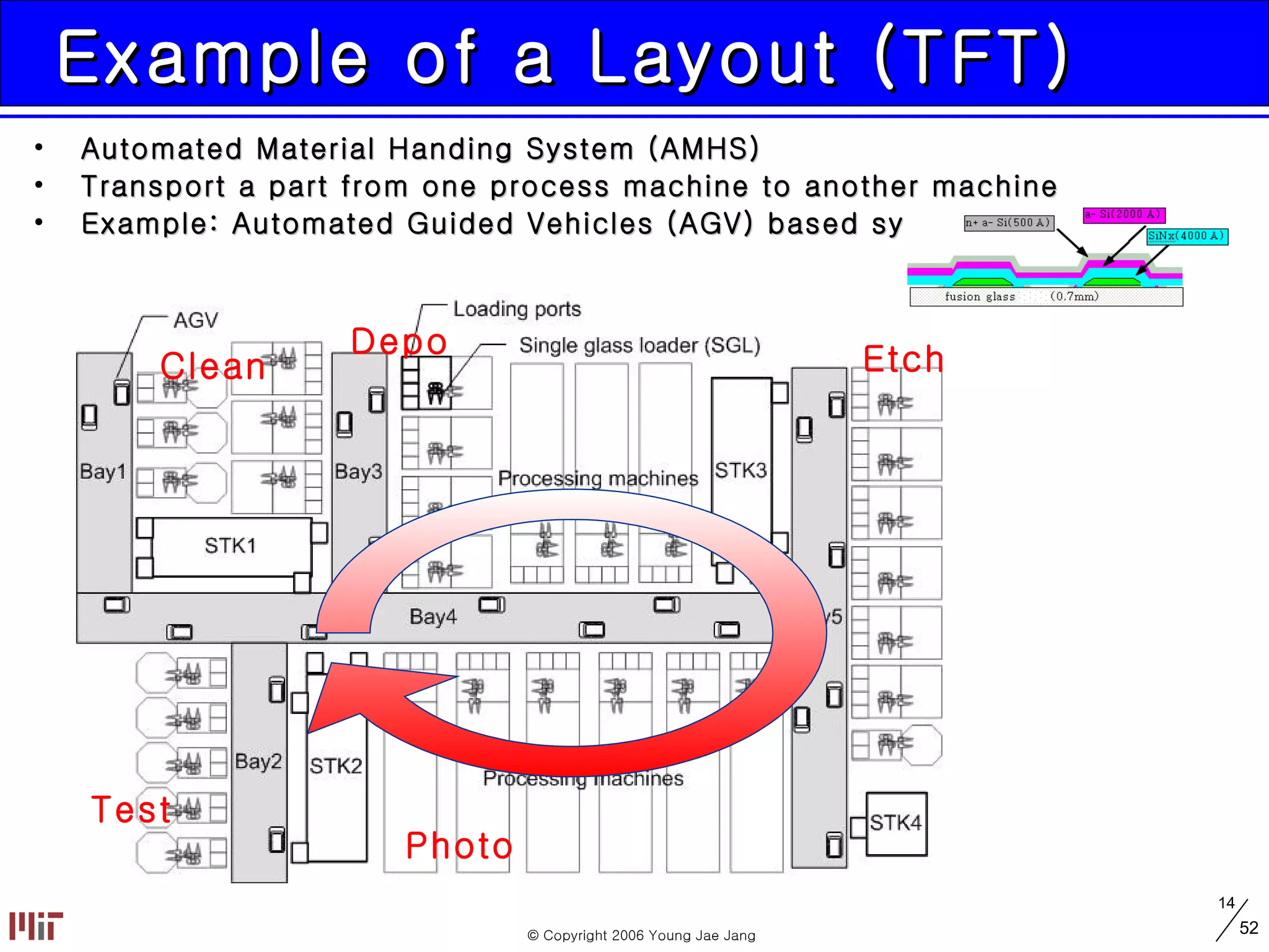
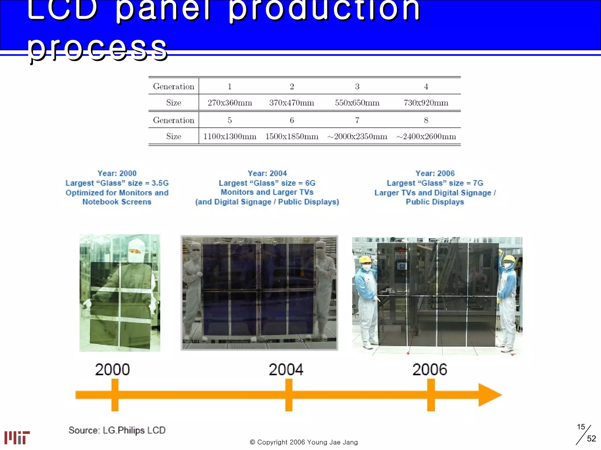
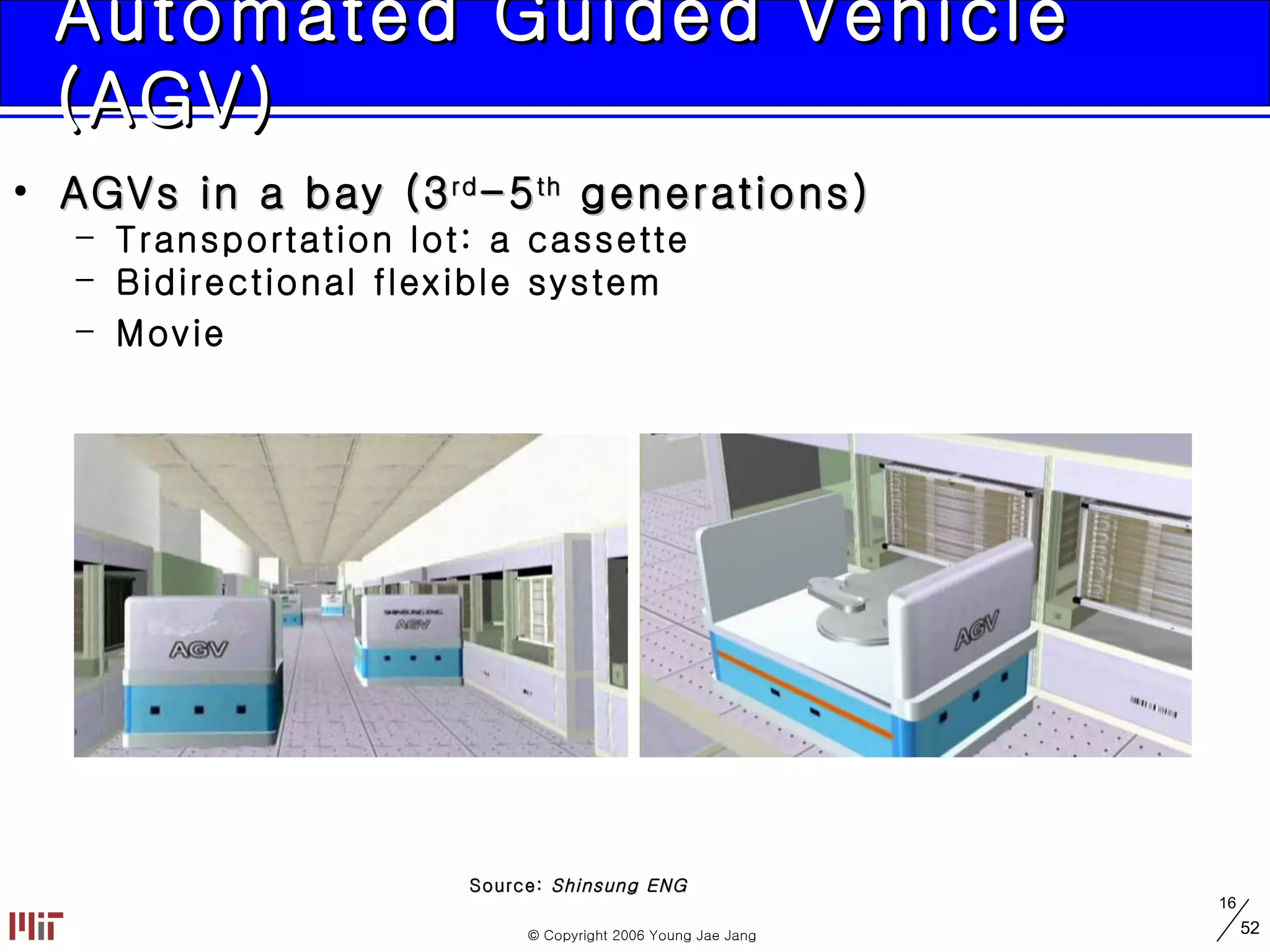
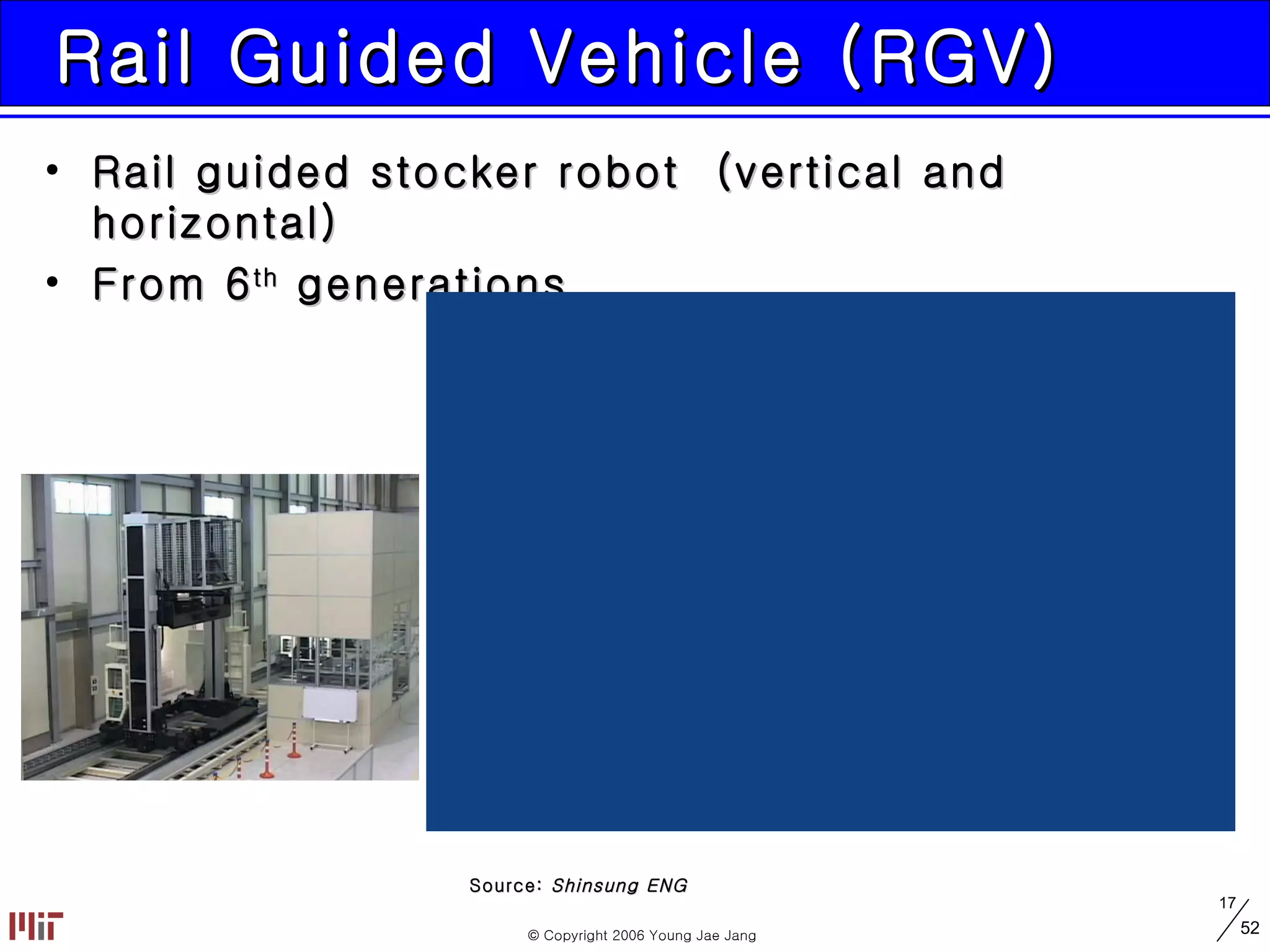
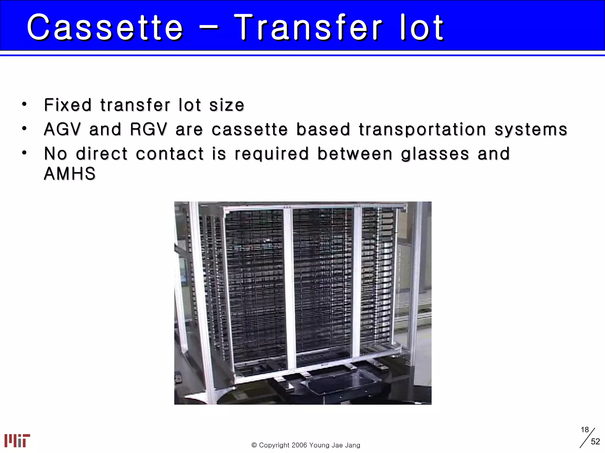
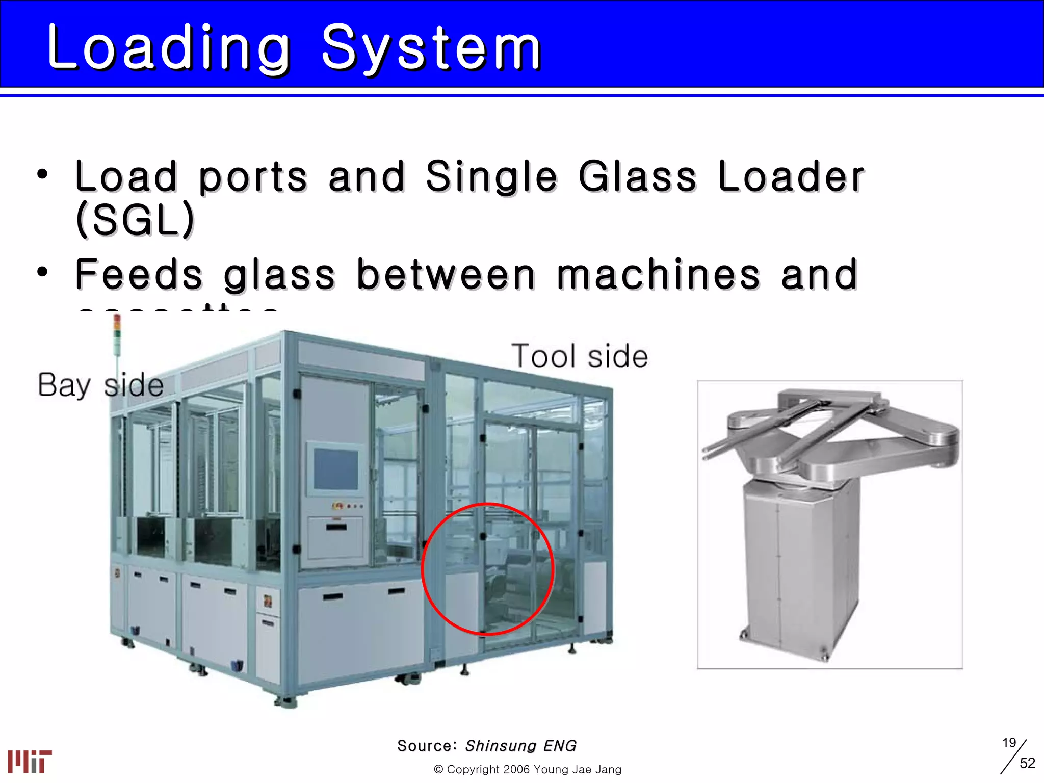
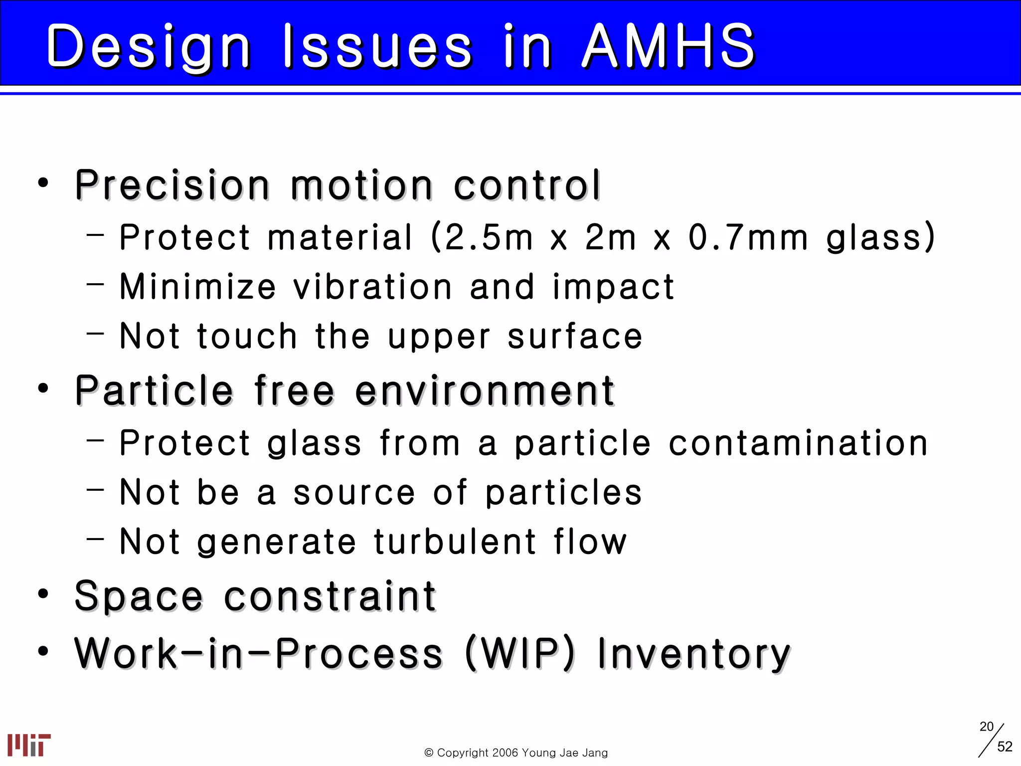
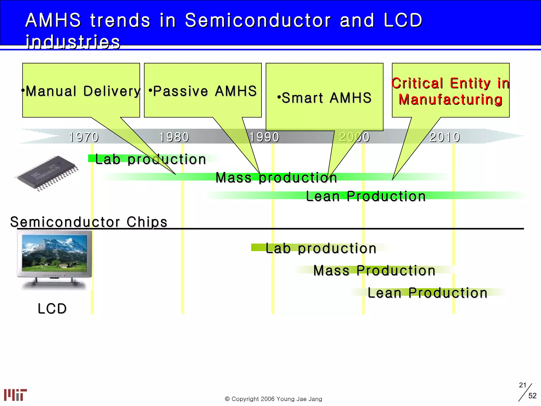
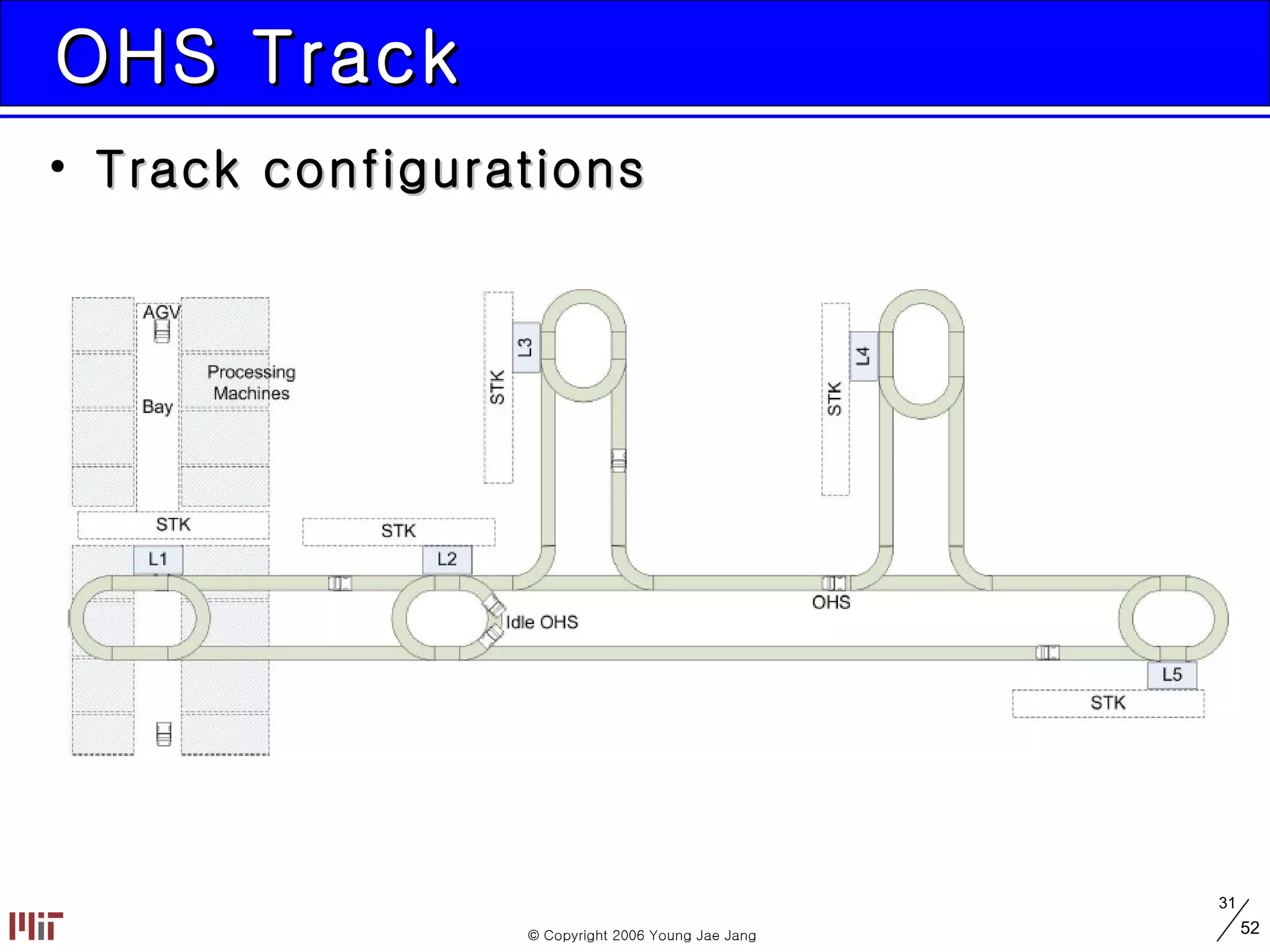
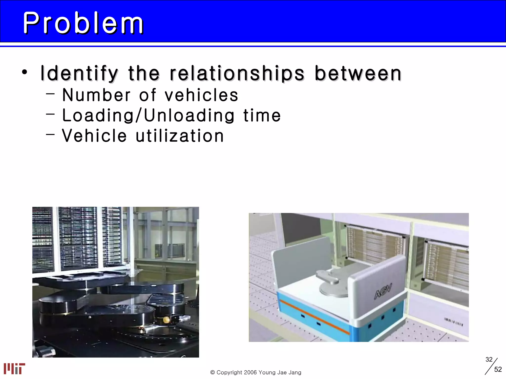
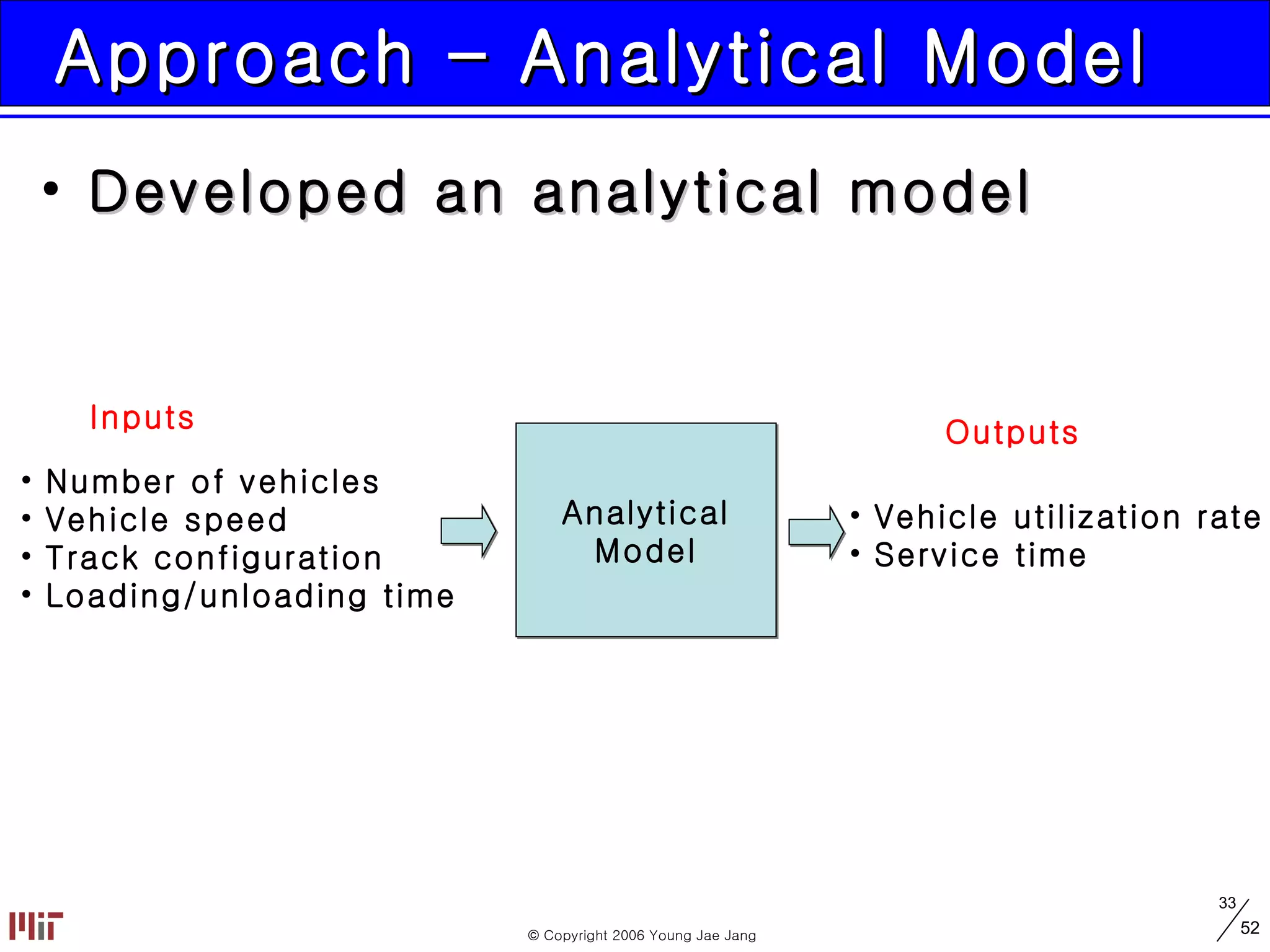
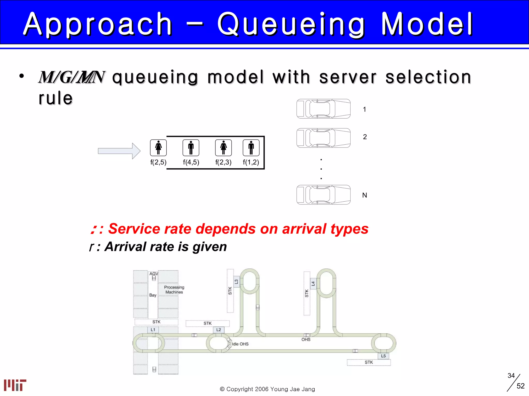
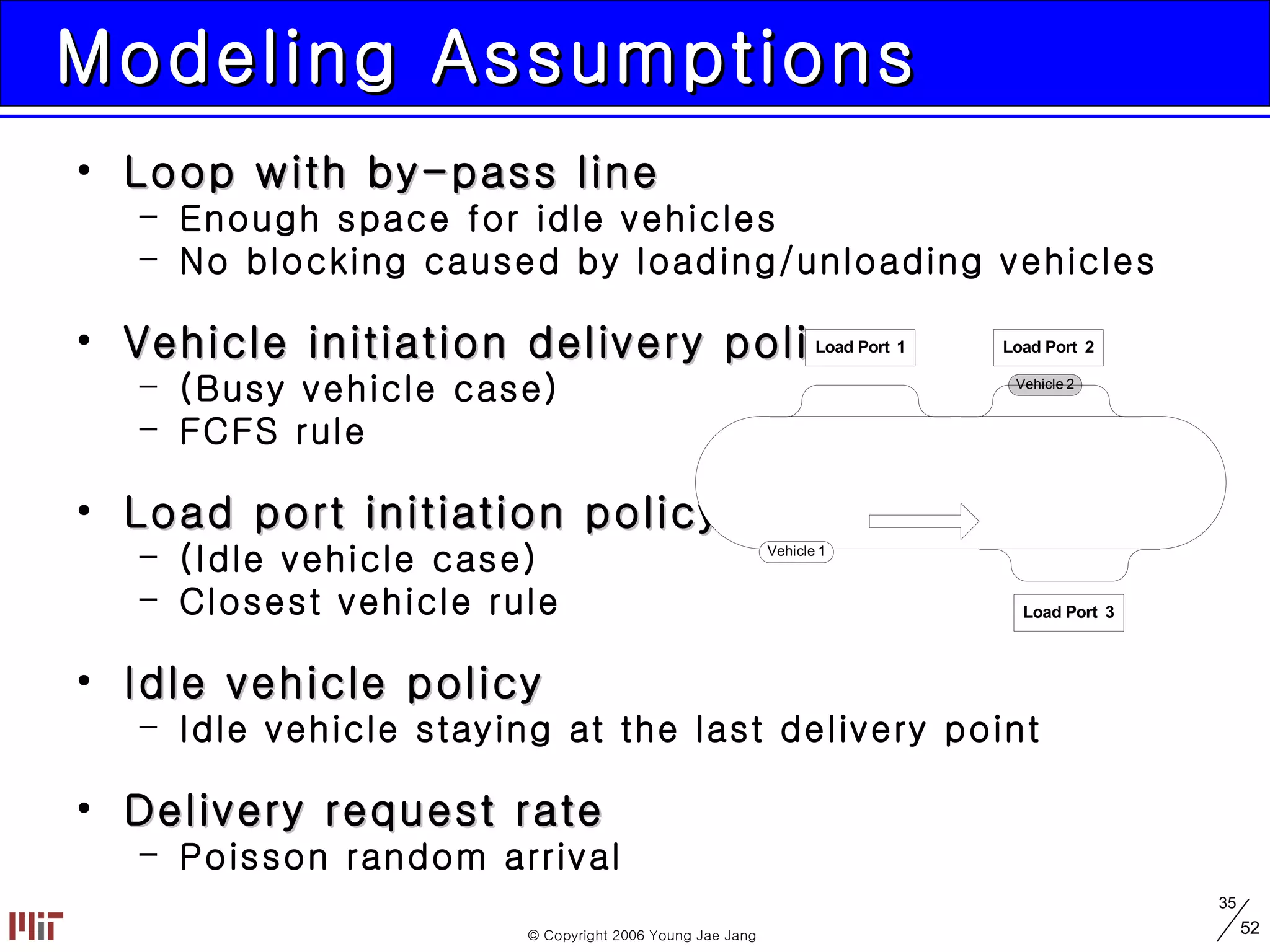
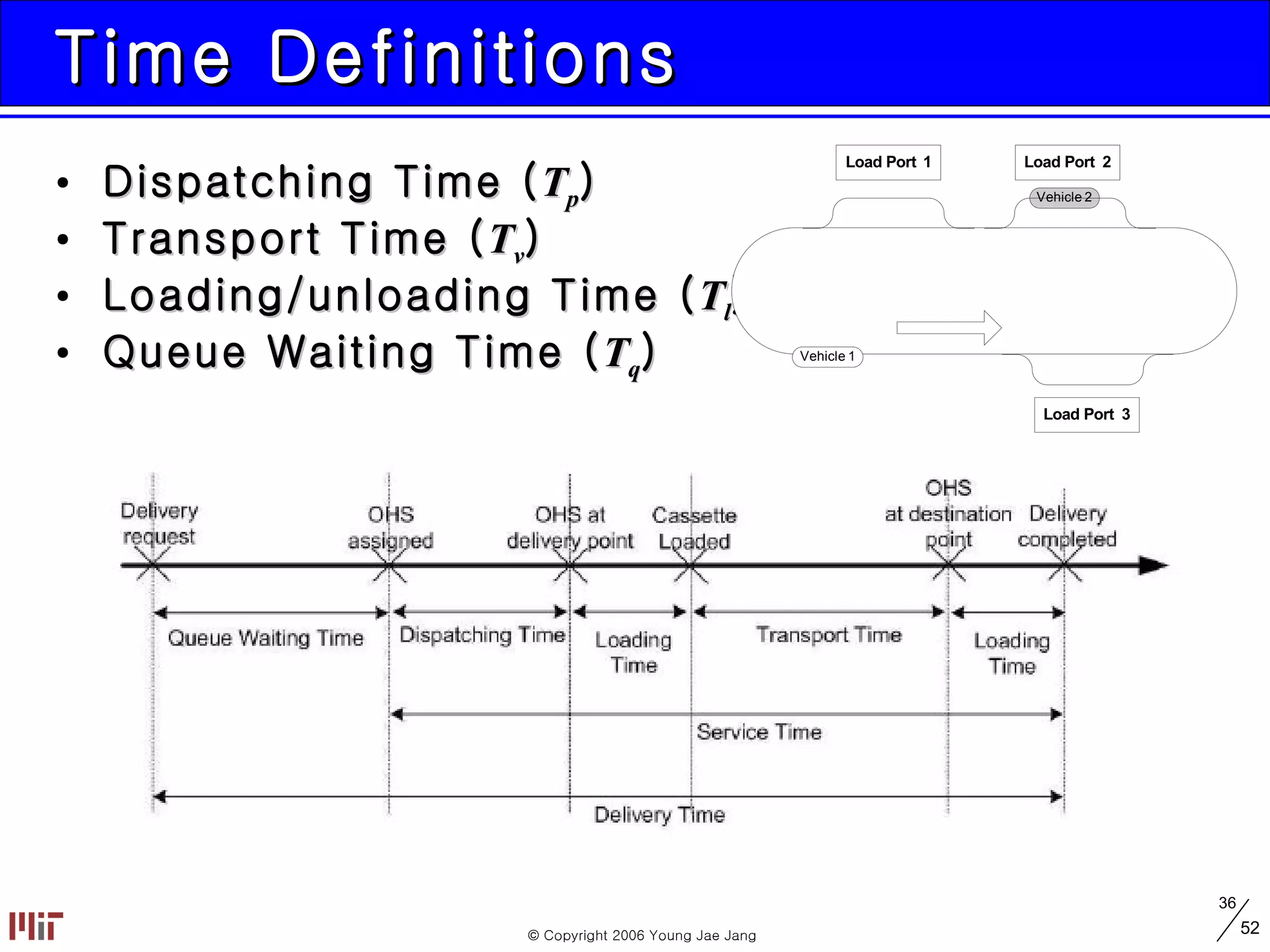
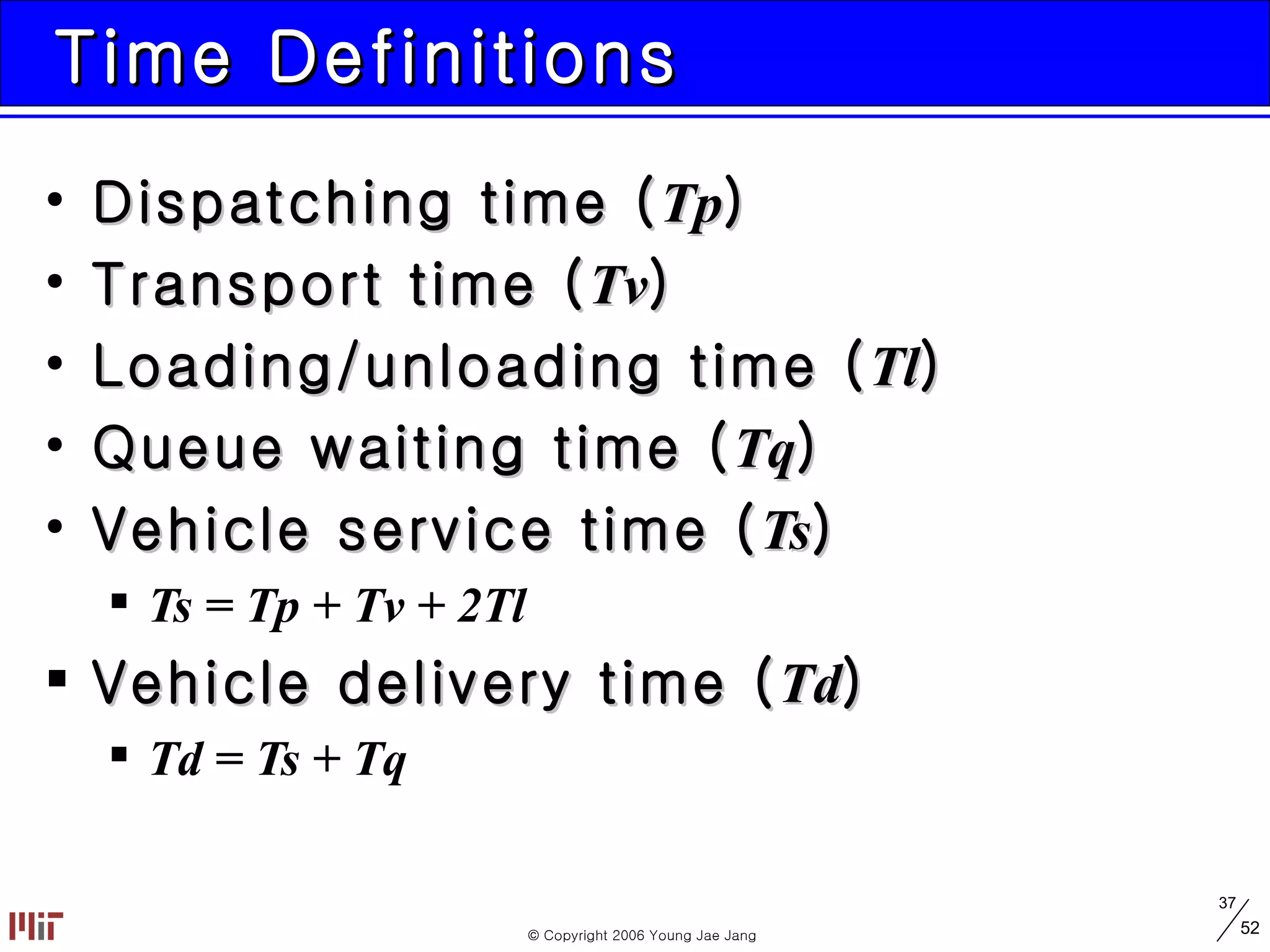
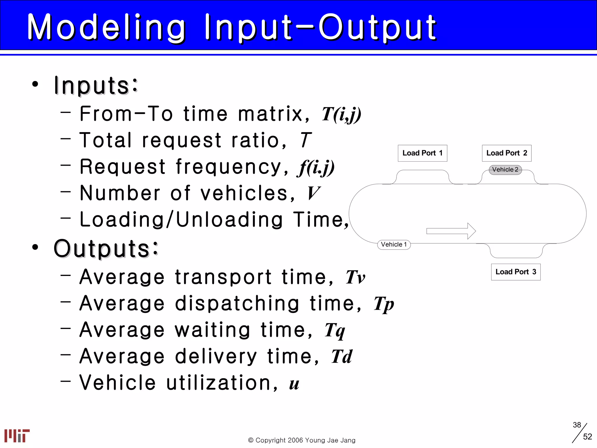
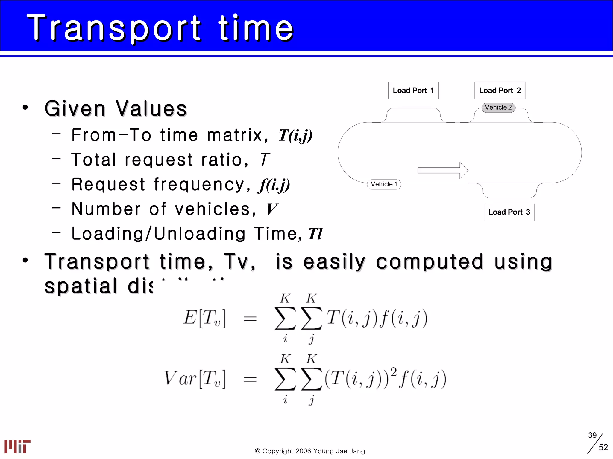
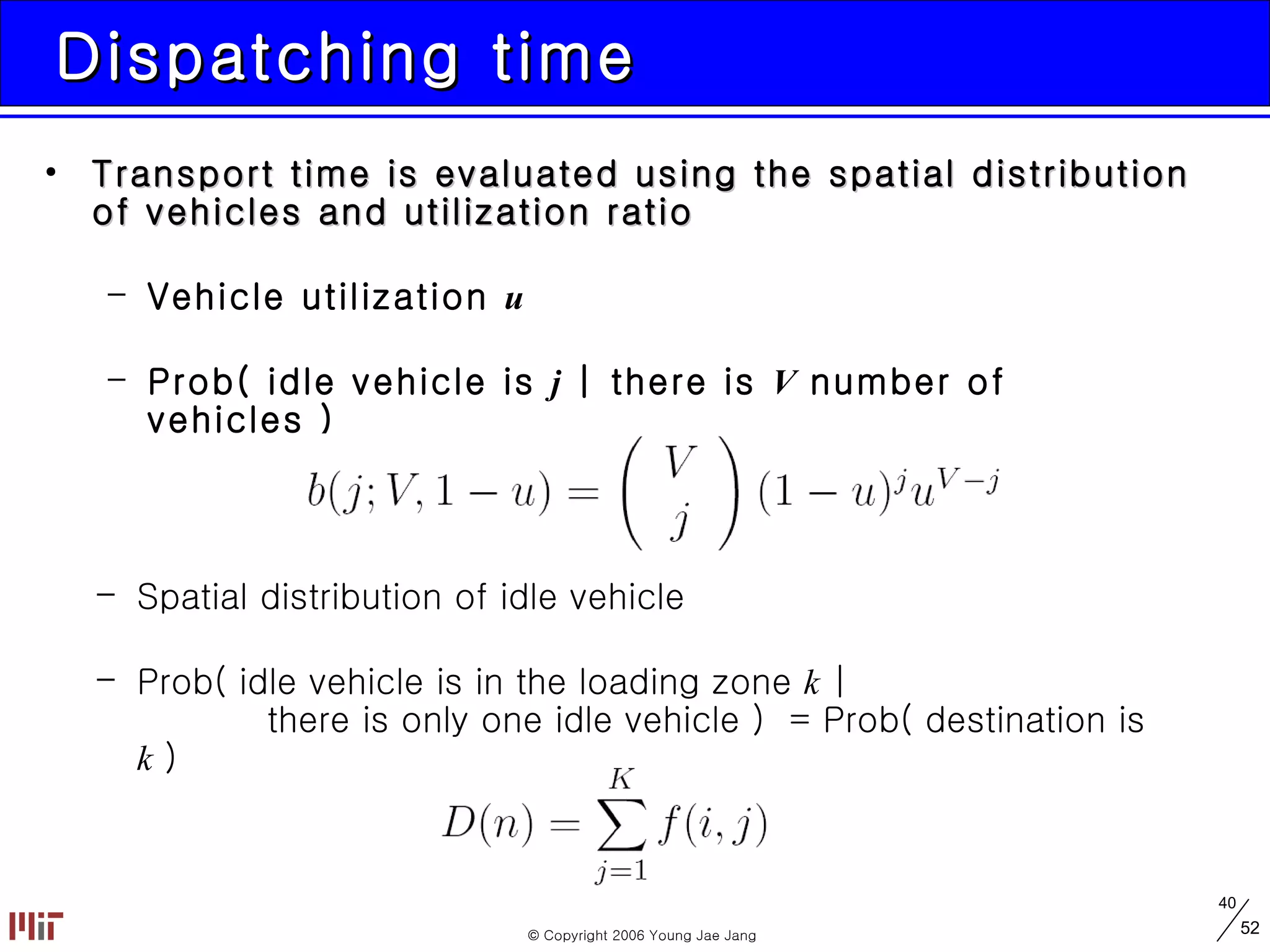
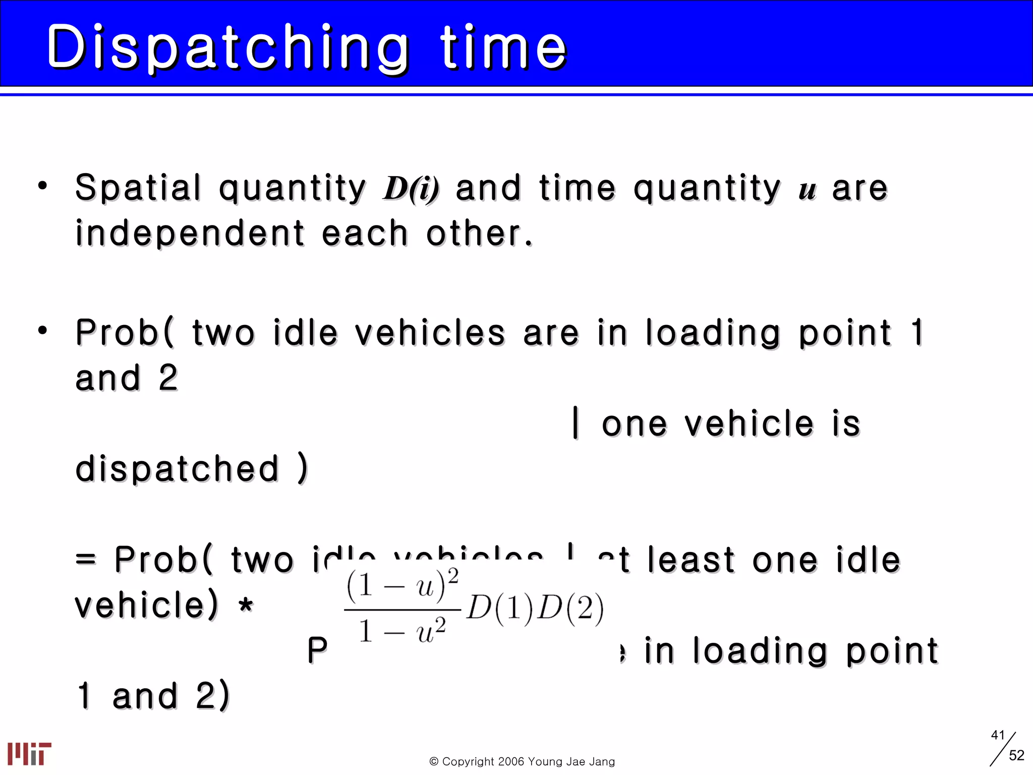
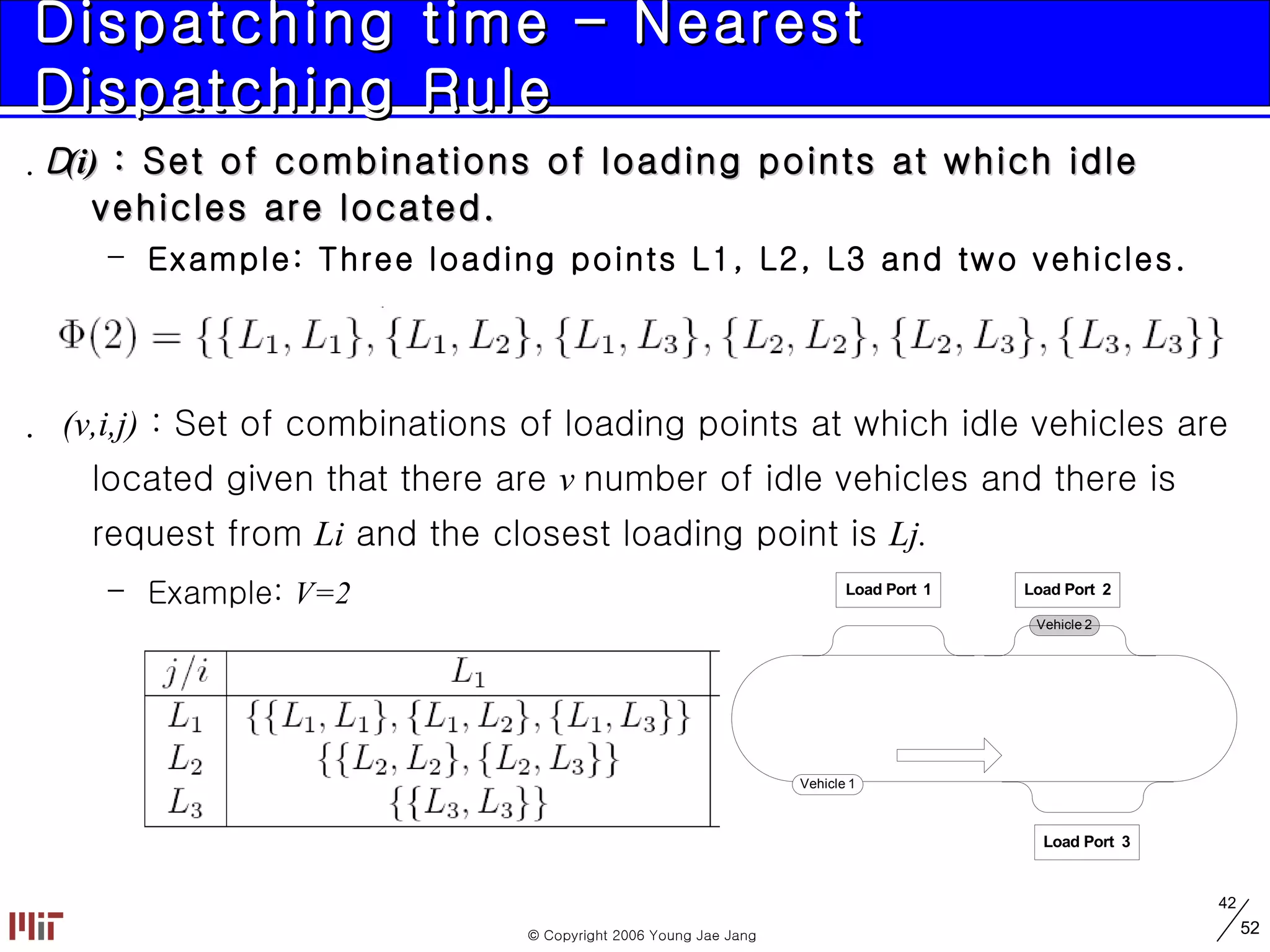
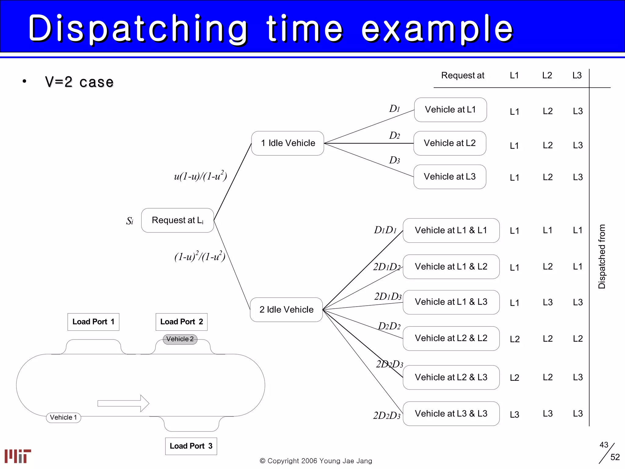
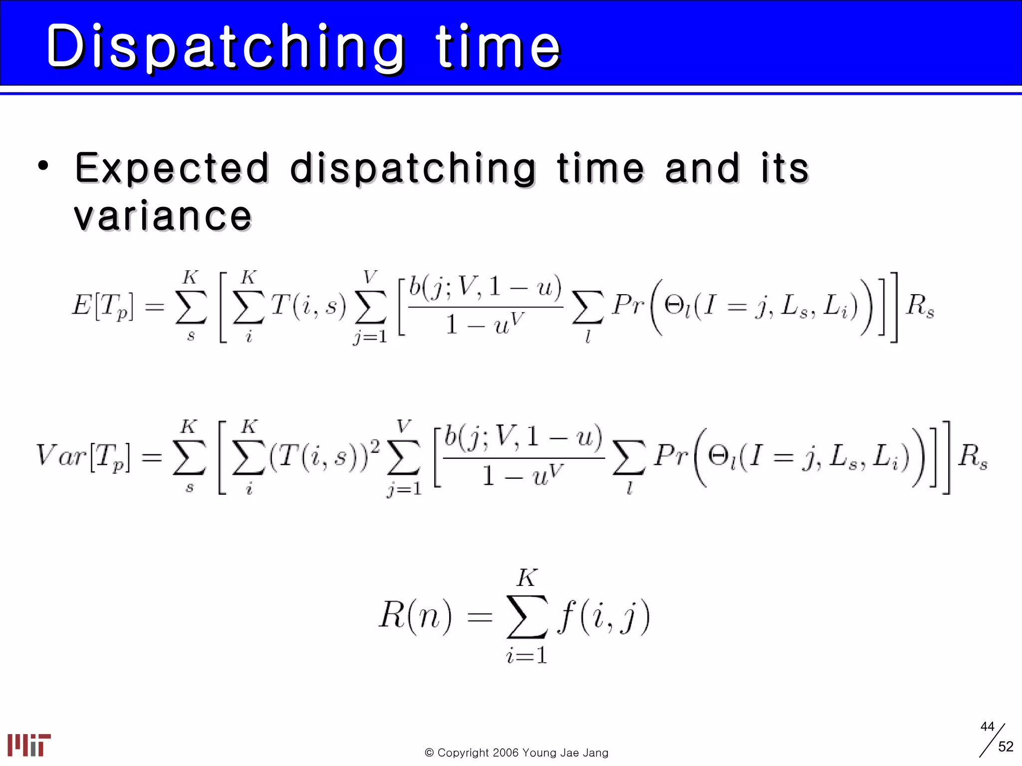
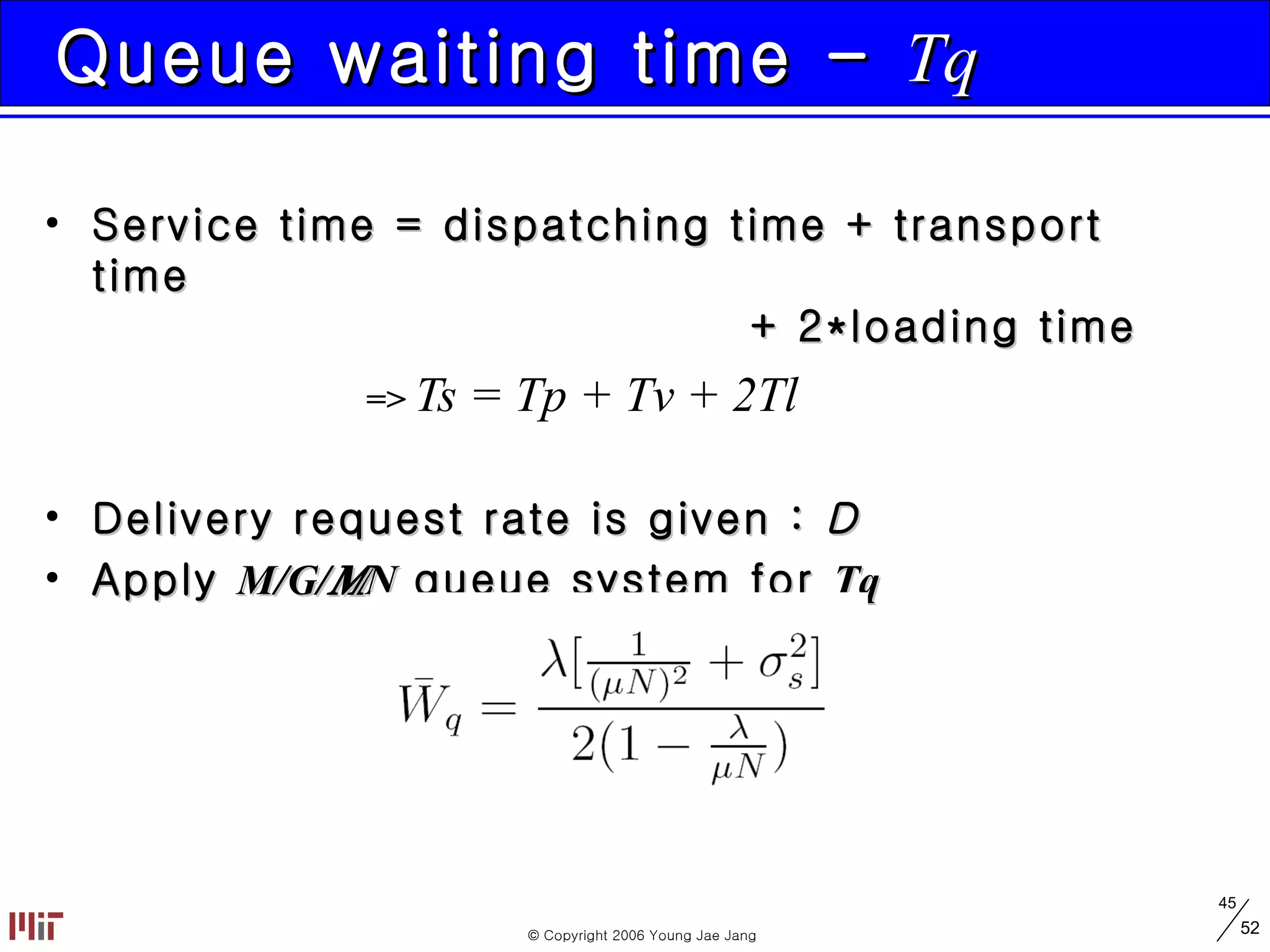
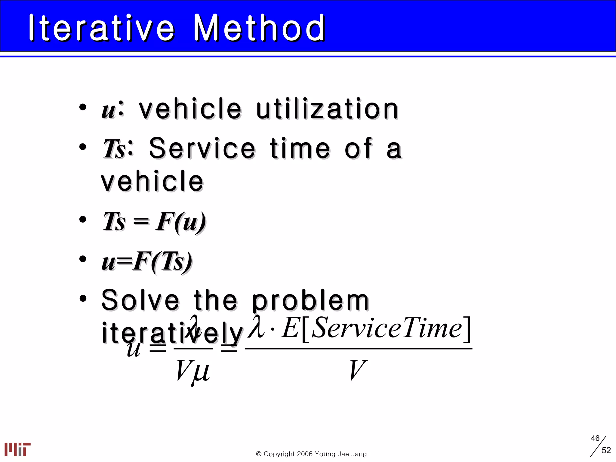
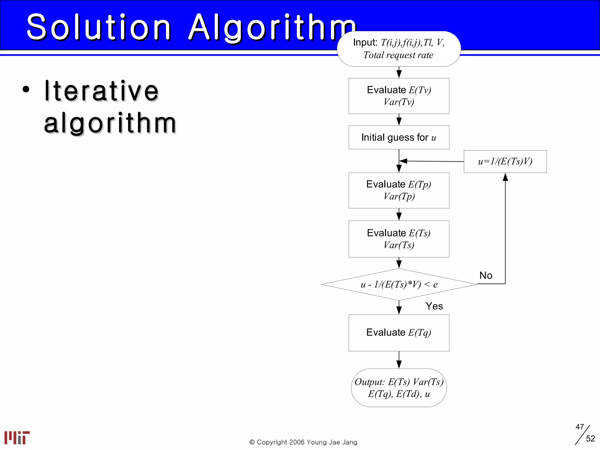
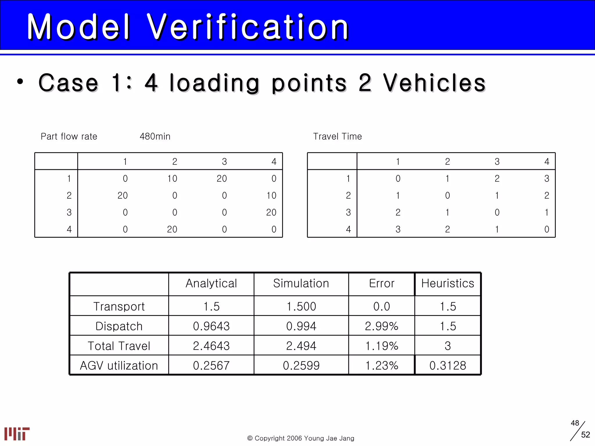
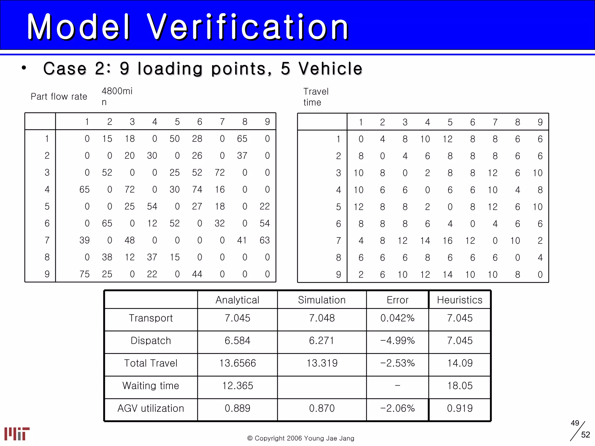
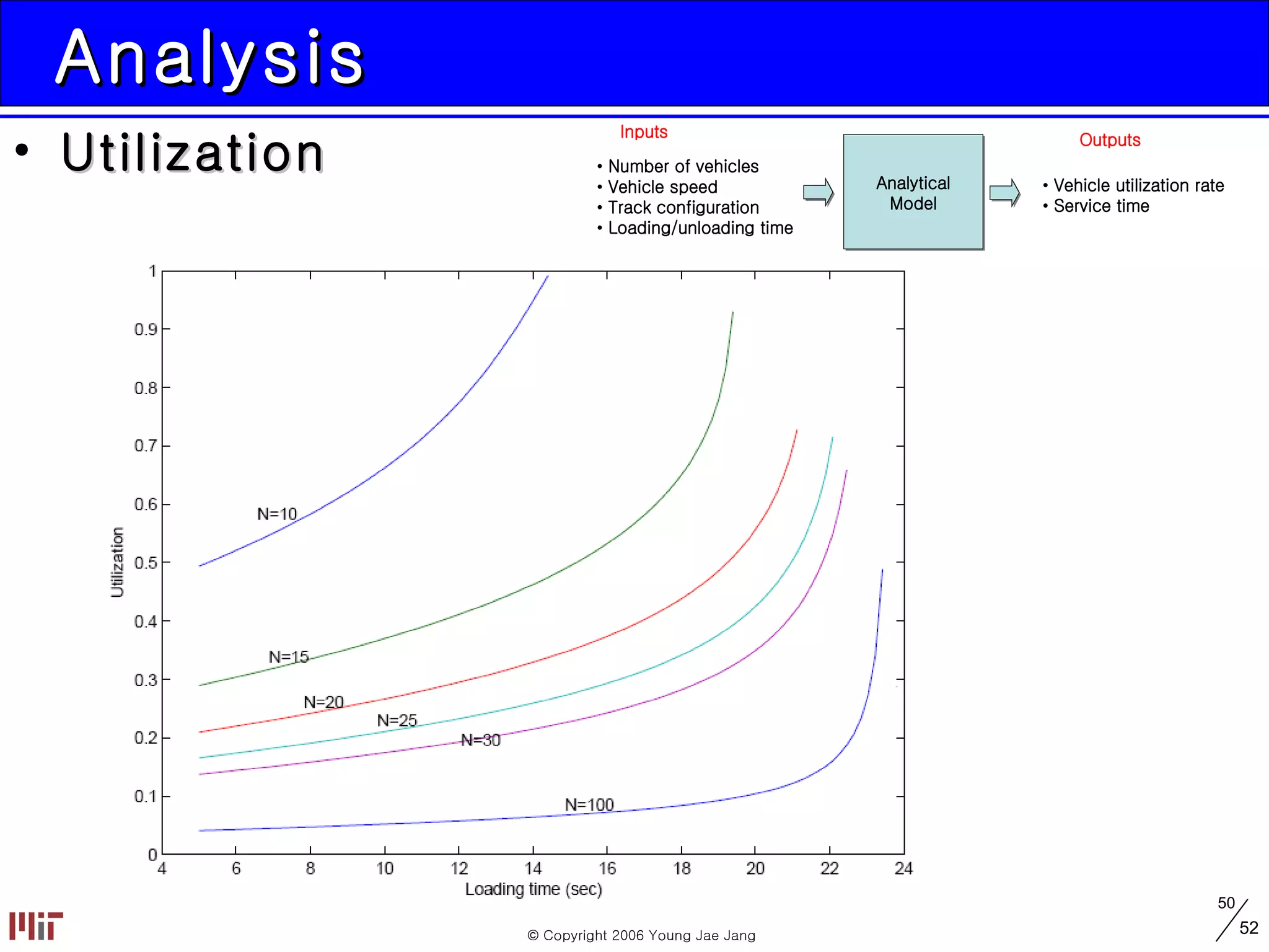
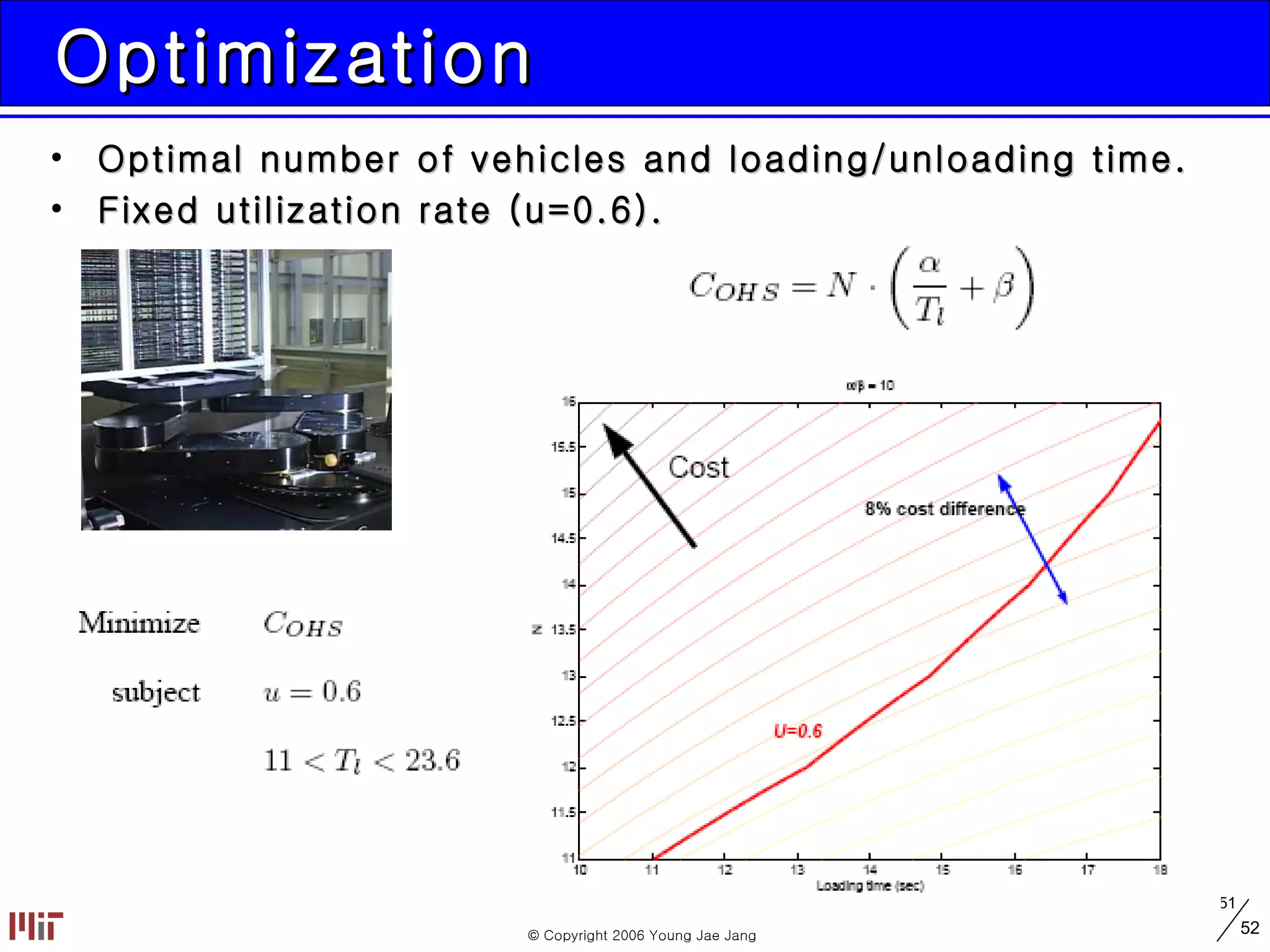
The document discusses automated material handling systems (AMHS) used in semiconductor and liquid crystal display (LCD) industries. It provides an overview of how AMHS are used in different stages of semiconductor wafer processing and LCD panel production. It also presents mathematical models to analyze AMHS, including queueing models to evaluate fleet size and vehicle utilization in AMHS.

1. Automated Material Handling Systems (AMHS) Young Jae Jang (youngjae@mit.edu) MIT December 11, 2006 2.853/2.854

2. Contents Introduction to AMHS AMHS in Semiconductor Industry AMHS in LCD industry Mathematical analysis in AMHS

3. Automated Material Handling Systems Automated material handling systems… Transfer parts from one place to another. Include conveyor belts, automated guided vehicles, rail guided vehicles etc. Used to be considered non-valued entities in manufacturing. Play a critical role in productivity in some industries. Semiconductor industry Liquid Crystal Display (LCD) industry M1 M2 B

4. AMHS Engineers Mechanical Engineering Disciplines. Control, Dynamics, and Robotics. Manufacturing Engineering Disciplines. Layout design, Track design, Optimizations, Scheduling, and so on. Example: Controller design and productivity Mechanical Engineering Manufacturing Engineering Material Handling System Engineering

5. Needs for AMHS Role of AMHS Supply chain Integration Real time control of manufacturing Low volume high product diversity Flexible Manufacturing Inventory WIP control Pull system High production rate Push system Low product diversity Laboratory No production strategy Production Strategy Real time communication with ERP system Advanced Production Advanced AMHS Flexible AMHS Flexible Production Passive AMHS Mass Production No Automations Birth of Industry AMHS Strategy Stage

6. AMHS trends in Semiconductor and LCD industries Lab production Mass production Lean Production Lab production Mass Production Lean Production Semiconductor Chips Manual Delivery Passive AMHS Smart AMHS Critical Entity in Manufacturing 1970 1980 1990 2000 2010 LCD

7. Contents Introduction to AMHS AMHS in Semiconductor Industry AMHS in LCD industry Mathematical analysis in AMHS

8. Semiconductor Manufacturing Front end – Wafer processing Back end – Chip packaging OHS – Overhead Shuttle System Cassette base system

9. AMHS in Semiconductor Fab OHS

10. Fleet Size Analysis – Simulations Solution 1 Layout Solution 2 Layout Solution 3 Layout AMHSA Layout

11. Fleet Size Analysis – Simulations 2/3

12. Contents Introduction to AMHS AMHS in Semiconductor Industry AMHS in LCD industry Mathematical analysis in AMHS

13. Main LCD Production Stages Similar to semiconductor device processes More than 200 processing steps – Three stages Array stage Transistors are fabricated on TFT glass Color Filter Layers is processed on C/F glass Cell stage TFT glass and C/F glass are joined The mother glass is cut into individual cells Liquid crystal is injected between the two glasses Module assembly stage Additional components, such as driver integrated circuits and backlight units, are connected Critical production Clean room environment TFT process C/F process Cell stage Module stage Array Stage C/F glass TFT glass Liquid Crystal

14. Example of a Layout (TFT) Automated Material Handing System (AMHS) Transport a part from one process machine to another machine Example: Automated Guided Vehicles (AGV) based system Photo Depo Etch Clean Test

15. LCD panel production process

16. Automated Guided Vehicle (AGV) AGVs in a bay (3 rd -5 th generations) Transportation lot: a cassette Bidirectional flexible system Movie Source: Shinsung ENG

17. Rail Guided Vehicle (RGV) Rail guided stocker robot (vertical and horizontal) From 6 th generations Source: Shinsung ENG

18. Cassette – Transfer lot Fixed transfer lot size AGV and RGV are cassette based transportation systems No direct contact is required between glasses and AMHS

19. Loading System Load ports and Single Glass Loader (SGL) Feeds glass between machines and cassettes Source: Shinsung ENG

20. Design Issues in AMHS Precision motion control Protect material (2.5m x 2m x 0.7mm glass) Minimize vibration and impact Not touch the upper surface Particle free environment Protect glass from a particle contamination Not be a source of particles Not generate turbulent flow Space constraint Work-in-Process (WIP) Inventory

21. AMHS trends in Semiconductor and LCD industries Lab production Mass production Lean Production Lab production Mass Production Lean Production Semiconductor Chips Manual Delivery Passive AMHS Smart AMHS Critical Entity in Manufacturing 1970 1980 1990 2000 2010 LCD

22. Current Market Situation Inventory issue: June 13, 2006 Its inventory has risen to four weeks of goods, unusually high in an industry accustomed to a one- to two-week range. LG.Philips took the unusual step of declaring that it would reduce volume for the rest of the quarter. In addition, "We are reviewing our total capacity plans for the year and beyond," Ron Wirahadiraksa, the company's president, said in a prepared statement. June , 15 2006 TAICHUNG, Taiwan -- AU Optronics Corp. has cut production of liquid-crystal displays because of bloated inventories , a move that could bring more stability to LCD prices by the third quarter if other companies follow suit, a company executive said.

23. Contents Introduction to AMHS AMHS in Semiconductor Industry AMHS in LCD industry Mathematical analysis in AMHS Case 1 – Buffer Allocation Case 2 – AMHS in LCD lines

24. Case 1 - Buffer Allocations Which one has higher production rate? 9 Machine line with two buffer options: This problem can be viewed as a bay structure with large stockers vs. unified structure with distributed I/O buffer in Fab

25. Decomposition Analysis – FAB design 8 buffers vs. 2 buffers, r=0.19, p=0.01, t=1

26. Results: Distributed buffer system in 300mm Fab

27. Contents Introduction to AMHS AMHS in Semiconductor Industry AMHS in LCD industry Mathematical analysis in AMHS Case 1 – Buffer Allocation Case 2 – AMHS in LCD lines

28. LCD – OHS System Development Overhead shuttle layout design and track design

29. OHS System Pilot system using linear motors

30. OHS Track Layout

31. OHS Track Track configurations

32. Problem Identify the relationships between Number of vehicles Loading/Unloading time Vehicle utilization

33. Approach – Analytical Model Developed an analytical model Analytical Model Number of vehicles Vehicle speed Track configuration Loading/unloading time Vehicle utilization rate Service time Inputs Outputs

34. Approach – Queueing Model M/G/  /N queueing model with server selection rule  : Arrival rate is given  : Service rate depends on arrival types

35. Modeling Assumptions Loop with by-pass line Enough space for idle vehicles No blocking caused by loading/unloading vehicles Vehicle initiation delivery policy (Busy vehicle case) FCFS rule Load port initiation policy (Idle vehicle case) Closest vehicle rule Idle vehicle policy Idle vehicle staying at the last delivery point Delivery request rate Poisson random arrival

36. Time Definitions Dispatching Time ( T p ) Transport Time ( T v ) Loading/unloading Time ( T l ) Queue Waiting Time ( T q )

37. Time Definitions Dispatching time ( Tp ) Transport time ( Tv ) Loading/unloading time ( Tl ) Queue waiting time ( Tq ) Vehicle service time ( Ts ) Ts = Tp + Tv + 2Tl Vehicle delivery time ( Td ) Td = Ts + Tq

38. Modeling Input-Output Inputs: From-To time matrix, T(i,j) Total request ratio,  Request frequency, f(i.j) Number of vehicles, V Loading/Unloading Time , Tl Outputs: Average transport time, Tv Average dispatching time, Tp Average waiting time, Tq Average delivery time, Td Vehicle utilization, u

39. Transport time Given Values From-To time matrix, T(i,j) Total request ratio,  Request frequency, f(i.j) Number of vehicles, V Loading/Unloading Time , Tl Transport time, Tv, is easily computed using spatial distribution

40. Dispatching time Transport time is evaluated using the spatial distribution of vehicles and utilization ratio Vehicle utilization u Prob( idle vehicle is j | there is V number of vehicles ) Spatial distribution of idle vehicle Prob( idle vehicle is in the loading zone k | there is only one idle vehicle ) = Prob( destination is k )

41. Dispatching time Spatial quantity D(i) and time quantity u are independent each other. Prob( two idle vehicles are in loading point 1 and 2 | one vehicle is dispatched ) = Prob( two idle vehicles | at least one idle vehicle) * Prob( vehicle are in loading point 1 and 2) =

42. Dispatching time – Nearest Dispatching Rule  (i) : Set of combinations of loading points at which idle vehicles are located. Example: Three loading points L1, L2, L3 and two vehicles.  (v,i,j) : Set of combinations of loading points at which idle vehicles are located given that there are v number of idle vehicles and there is request from Li and the closest loading point is Lj. Example: V=2

43. Dispatching time example V=2 case

44. Dispatching time Expected dispatching time and its variance

45. Queue waiting time - Tq Service time = dispatching time + transport time + 2*loading time => Ts = Tp + Tv + 2Tl Delivery request rate is given :  Apply M/G/  /N queue system for Tq

46. Iterative Method u : vehicle utilization Ts : Service time of a vehicle Ts = F(u) u=F(Ts) Solve the problem iteratively

47. Solution Algorithm Iterative algorithm

48. Model Verification Case 1: 4 loading points 2 Vehicles 1.23% 1.19% 2.99% 0.0 Error AGV utilization Total Travel Dispatch Transport 0.3128 0.2599 0.2567 3 2.494 2.4643 1.5 0.994 0.9643 1.5 1.500 1.5 Heuristics Simulation Analytical 0 0 20 0 4 20 0 0 0 3 10 0 0 20 2 0 20 10 0 1 4 3 2 1 480min Part flow rate 0 1 2 3 4 1 0 1 2 3 2 1 0 1 2 3 2 1 0 1 4 3 2 1 Travel Time

49. Model Verification Case 2: 9 loading points, 5 Vehicle 14.09 -2.53% 13.319 13.6566 Total Travel -2.06% - -4.99% 0.042% Error AGV utilization Waiting time Dispatch Transport 0.919 0.870 0.889 18.05 12.365 7.045 6.271 6.584 7.045 7.048 7.045 Heuristics Simulation Analytical 0 0 0 44 0 22 0 25 75 9 0 0 0 0 15 37 12 38 0 8 63 41 0 0 0 0 48 0 39 7 54 0 32 0 52 12 0 65 0 6 22 0 18 27 0 54 25 0 0 5 0 0 16 74 30 0 72 0 65 4 0 0 72 52 25 0 0 52 0 3 0 37 0 26 0 30 20 0 0 2 0 65 0 28 50 0 18 15 0 1 9 8 7 6 5 4 3 2 1 4800min Part flow rate 0 8 10 10 14 12 10 6 2 9 4 0 6 6 6 8 6 6 6 8 2 10 0 12 16 14 12 8 4 7 6 6 4 0 4 6 8 8 8 6 10 6 12 8 0 2 8 8 12 5 8 4 10 6 6 0 6 6 10 4 10 6 12 8 8 2 0 8 10 3 6 6 8 8 8 6 4 0 8 2 6 6 8 8 12 10 8 4 0 1 9 8 7 6 5 4 3 2 1 Travel time

50. Analysis Utilization

51. Optimization Optimal number of vehicles and loading/unloading time. Fixed utilization rate (u=0.6).

52. Conclusions AMHS becomes an important part in manufacturing systems. In semiconductor and LCD industries, AMHS plays a critical role in the productivity. Analysis for AMHS is often performed with simulations. Analytical models can provide AMHS engineers with intuition and understanding of the dynamic behavior of the system.