Downloaded 2,867 times

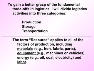
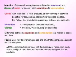
![Logistics – Mission [A Bill of “Rights”] Logistics embodies the effort to deliver: the right product in the right quantity in the right condition to the right place at the right time for the right customer at the right cost](https://image.slidesharecdn.com/mathi03-12520694134145-phpapp03/85/LOGISTICS-PLANNING-11-320.jpg)
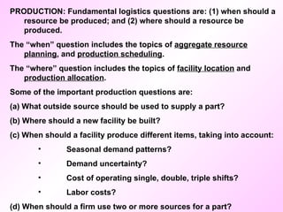
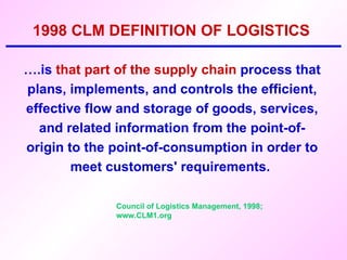
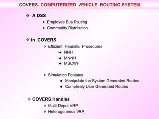
![Single-mode Service Choices and Issues Air Rapidly growing segment of transportation industry Lightweight, small items [Products: Perishable and time sensitive goods: Flowers, produce, electronics, mail, emergency shipments, documents, etc.] Quick, reliable, expensive Often combined with trucking operations Rail Low cost, high-volume [Products: Heavy industry, minerals, chemicals, agricultural products, autos, etc.] Improving flexibility intermodal service Truck Most used mode Flexible, small loads [Products: Medium and light manufacturing, food, clothing, all retail goods] Trucks can go door-to-door as opposed to planes and trains.](https://image.slidesharecdn.com/mathi03-12520694134145-phpapp03/85/LOGISTICS-PLANNING-17-320.jpg)
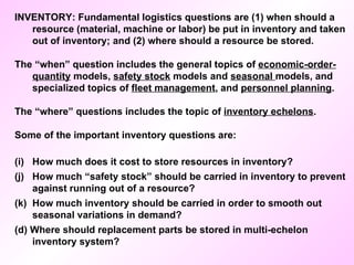
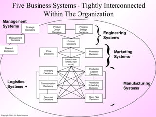
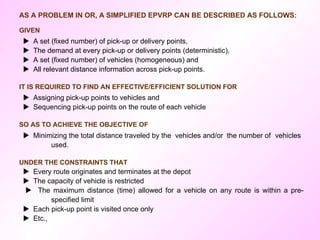
![Single-mode Service Choices and Issues (Contd.) Water One of oldest means of transport Low-cost, high-volume, slow Bulky, heavy and/or large items (Products: Nonperishable bulk cargo - Liquids, minerals, grain, petroleum, lumber, etc )] Standardized shipping containers improve service Combined with trucking & rail for complete systems International trade Pipeline Primarily for oil & refined oil products Slurry lines carry coal or kaolin High capital investment Low operating costs Can cross difficult terrain Highly reliable; Low product losses](https://image.slidesharecdn.com/mathi03-12520694134145-phpapp03/85/LOGISTICS-PLANNING-18-320.jpg)
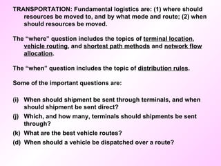
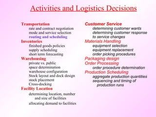
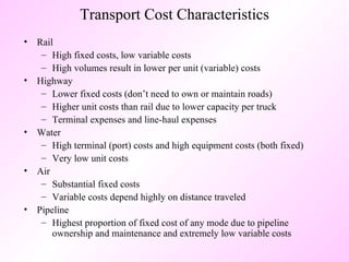
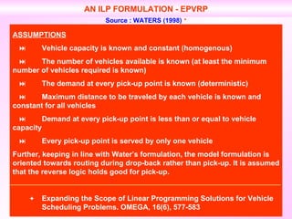
![Transport Cost Characteristics Fixed costs: Terminal facilities Transport equipment Carrier administration Roadway acquisition and maintenance [ Infrastructure (road, rail, pipeline, navigation, etc.)] Variable costs: Fuel Labor Equipment maintenance Handling, pickup & delivery, taxes NOTE : Cost structure varies by mode](https://image.slidesharecdn.com/mathi03-12520694134145-phpapp03/85/LOGISTICS-PLANNING-19-320.jpg)
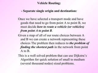
![Suppose we have multiple sources and multiple destinations , that each destination requires some integer number of truckloads, and that none of the sources have capacity restrictions [ No Capacity Restriction ]. In this case we can simply apply the transportation method of linear programming to determine the assignment of sources to destinations. Vehicle Routing: - Multiple Origin and Destination Points Sources Destinations](https://image.slidesharecdn.com/mathi03-12520694134145-phpapp03/85/LOGISTICS-PLANNING-22-320.jpg)
![E MPLOYEE P ICKUP V E HICLE R OUTING P ROBLEM (EPVRP) – BANGALORE, KARNATAKA, INDIA Indian Telephone Industries [ITI] Limited Bharat Electronics Limited [BEL] Hindustan Machine Tools [HMT] Hindustan Aeronautics Limited [HAL] Indian Space Research Organization [ISRO] National Aeronautical Laboratory [NAL] Central Machine Tools of India [CMTI] ………](https://image.slidesharecdn.com/mathi03-12520694134145-phpapp03/85/LOGISTICS-PLANNING-35-320.jpg)
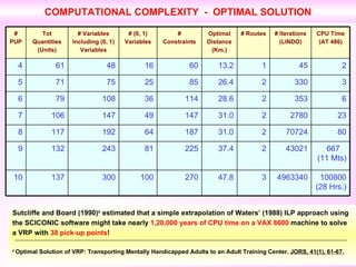
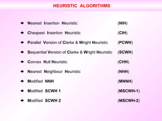
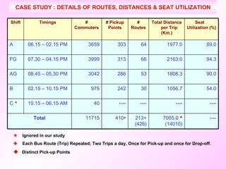
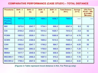
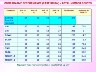
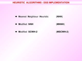
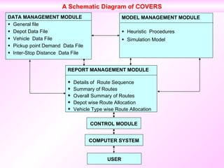


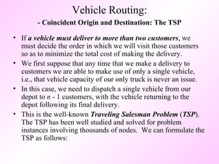
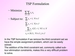
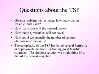
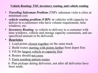
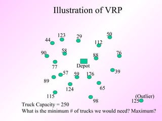
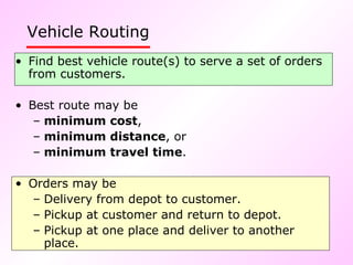
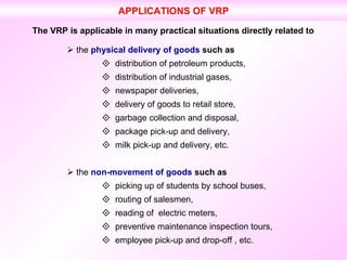
This document summarizes key aspects of vehicle routing problems (VRP). It discusses the traveling salesman problem (TSP) as a special case of VRP where a single vehicle must visit multiple locations. It also describes more complex VRP formulations that involve multiple vehicles with capacity constraints serving multiple customers. Heuristics for constructing initial feasible routes and improving routes are described. Finally, an example employee pickup VRP problem in Bangalore, India is presented to illustrate a real-world application of VRP.