DSS

1. Contents
2
 Hardware modeling:
 Switch level modeling
 Gate (structural) level modeling
 Behavioral modeling
 Module instantiation
 Assignments
 Procedural blocks
 Conditional and loop constructs
 Timing control
 Compiler directives and system
tasks
 T
asks and functions
 Basic testbench

2. Tools we will use
3
Editor (optional) HDL Designer
Simulator Mentor Modelsim
Synthesis Synopsys Design Compiler (Linux) – dc-
shell; Quartus (optional)

3. Simulation algorithms
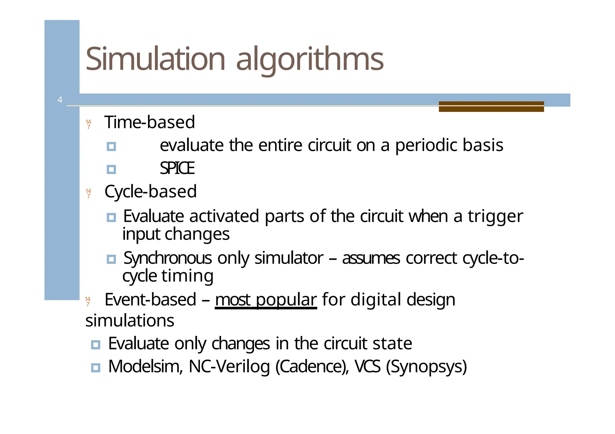
 Time-based
🞑 evaluate the entire circuit on a periodic basis
🞑 SPICE
 Cycle-based
🞑 Evaluate activated parts of the circuit when a trigger
input changes
🞑 Synchronous only simulator – assumes correct cycle-to-
cycle timing
 Event-based – most popular for digital design
simulations
🞑 Evaluate only changes in the circuit state
🞑 Modelsim, NC-Verilog (Cadence), VCS (Synopsys)
4

4. Modeling concurrency
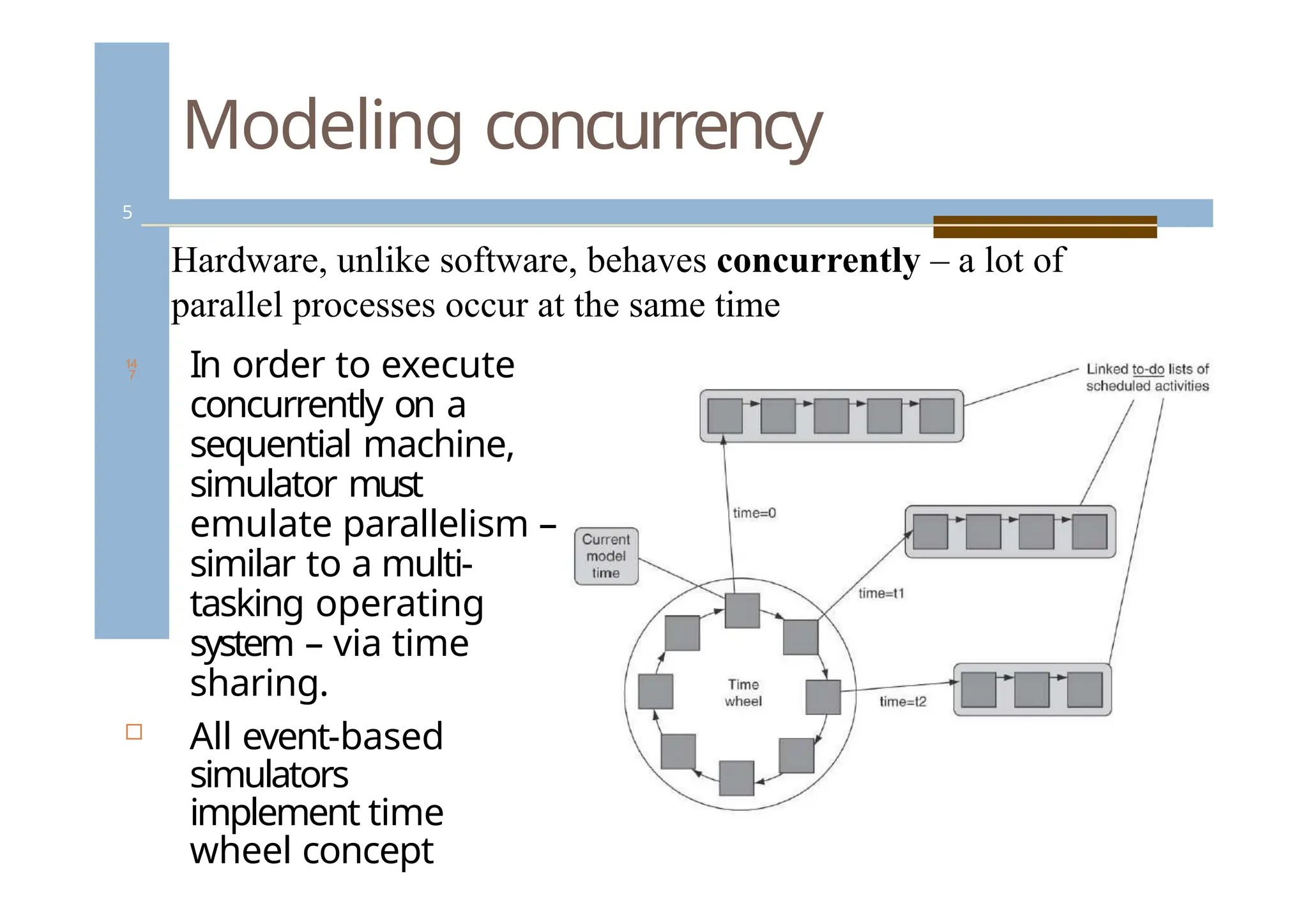
Hardware, unlike software, behaves concurrently – a lot of
parallel processes occur at the same time
 In order to execute
concurrently on a
sequential machine,
simulator must
emulate parallelism –
similar to a multi-
tasking operating
system – via time
sharing.
 All event-based
simulators
implement time
wheel concept
5

5. Modeling concurrency
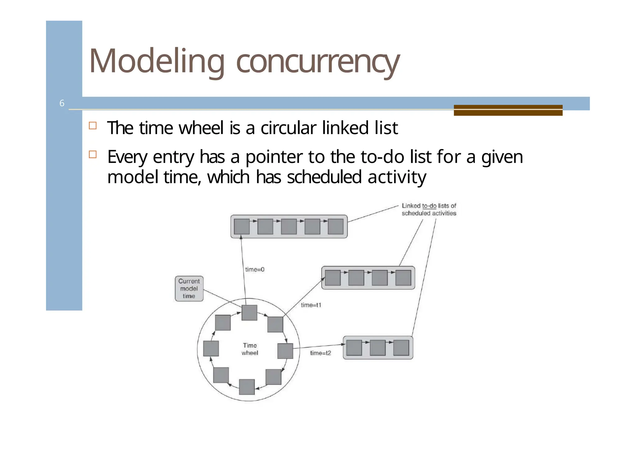
 The time wheel is a circular linked list
 Every entry has a pointer to the to-do list for a given
model time, which has scheduled activity
6

6. Modeling concurrency - simulation time
wheel
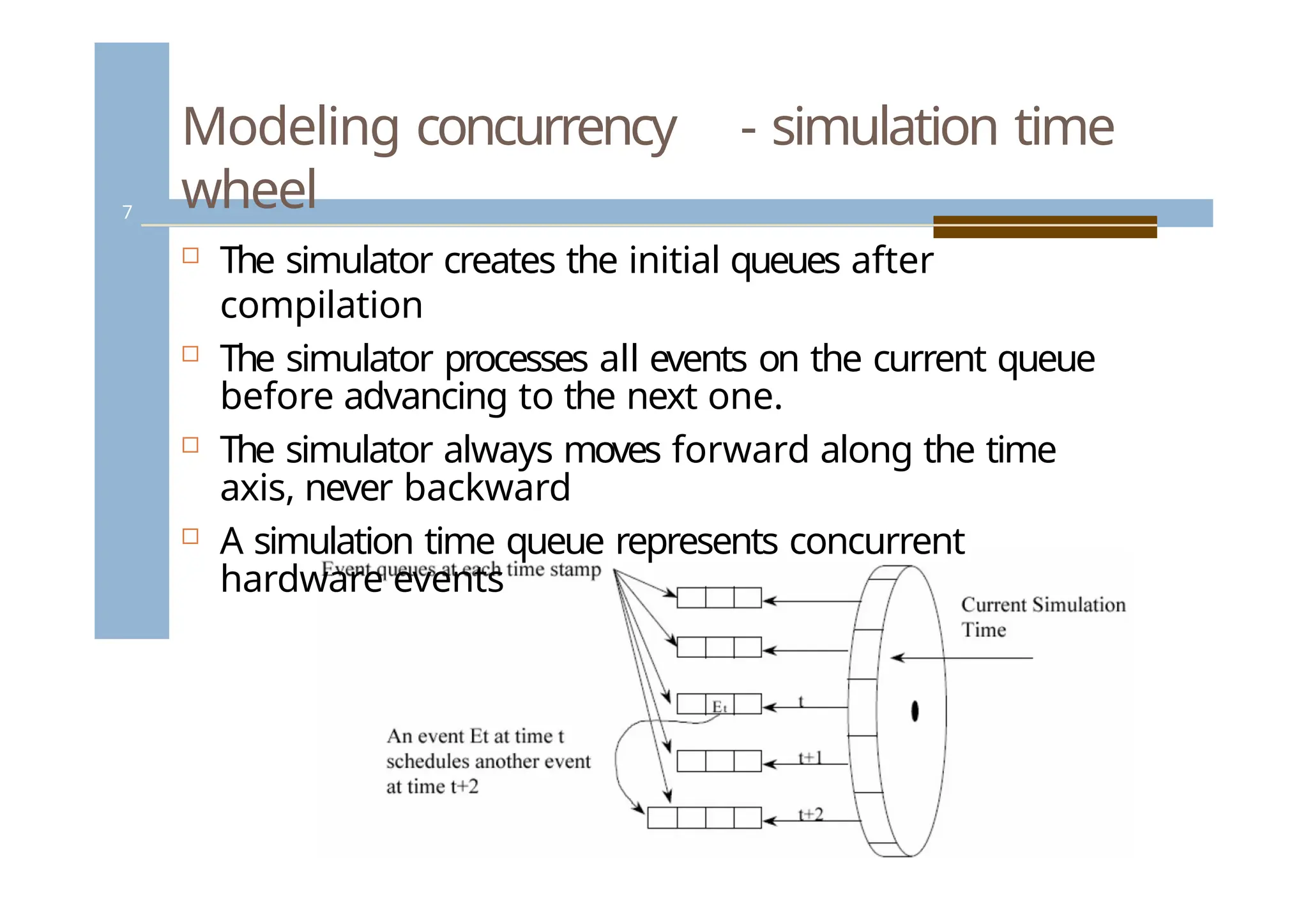
 The simulator creates the initial queues after
compilation
 The simulator processes all events on the current queue
before advancing to the next one.
 The simulator always moves forward along the time
axis, never backward
 A simulation time queue represents concurrent
hardware events
7

7. Verilog race condition
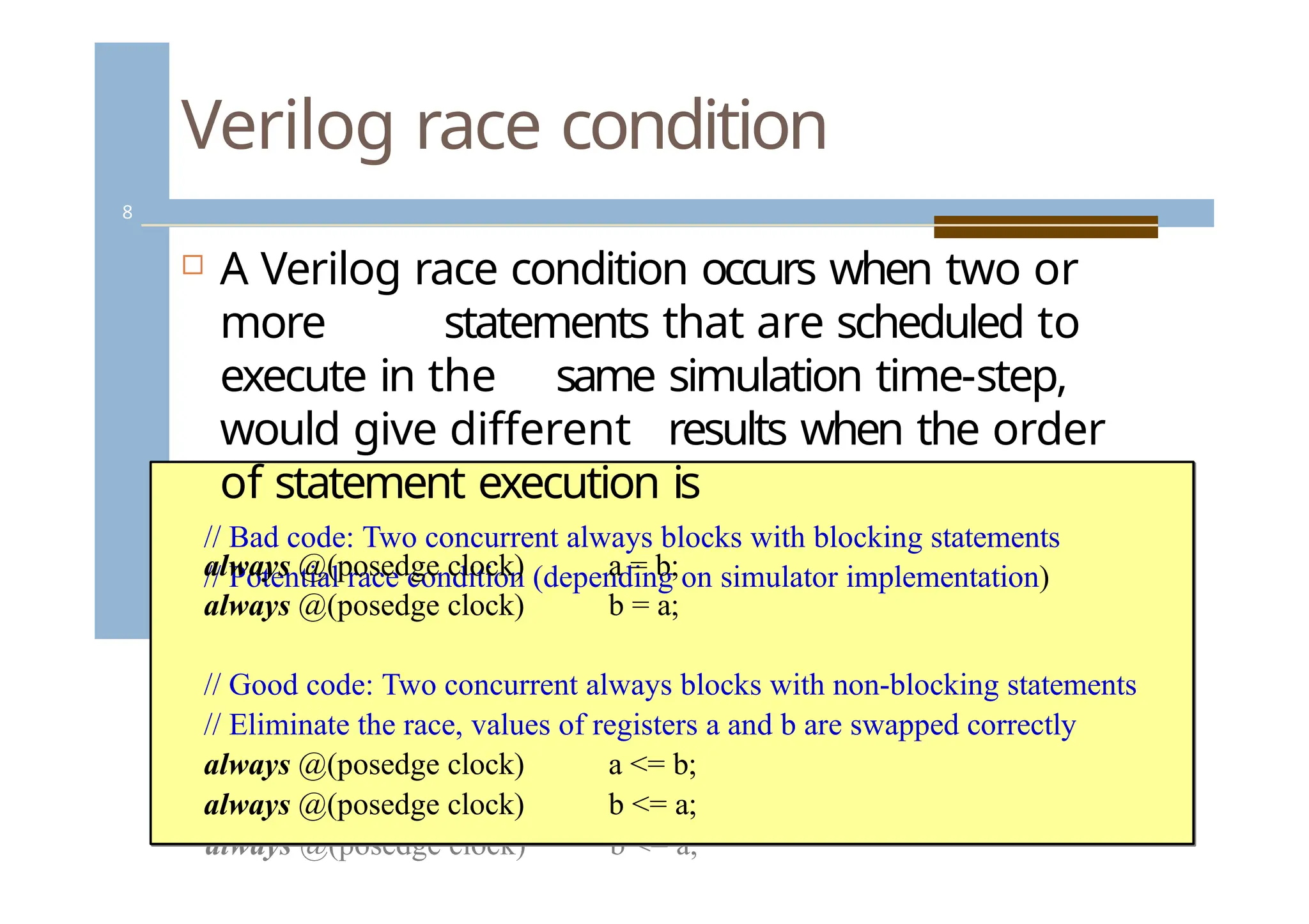
//cBhaadncogdee:dT.wo concurrent always blocks with blocking statements
// Potential race condition (depending on simulator implementation)
always @(posedge clock) a = b;
always @(posedge clock) b = a;
// Good code: Two concurrent always blocks with non-blocking
statements
// Eliminate the race, values of registers a and b are swapped correctly
always @(posedge clock) a <= b;
always @(posedge clock) b <= a;
 A Verilog race condition occurs when two or
more statements that are scheduled to
execute in the same simulation time-step,
would give different results when the order
of statement execution is
// Bad code: Two concurrent always blocks with blocking statements
// Potential race condition (depending on simulator implementation)
always @(posedge clock)
always @(posedge clock)
a = b;
b = a;
// Good code: Two concurrent always blocks with non-blocking statements
// Eliminate the race, values of registers a and b are swapped correctly
always @(posedge clock)
always @(posedge clock)
a <= b;
b <= a;
8

8. Switch Level Modeling
9
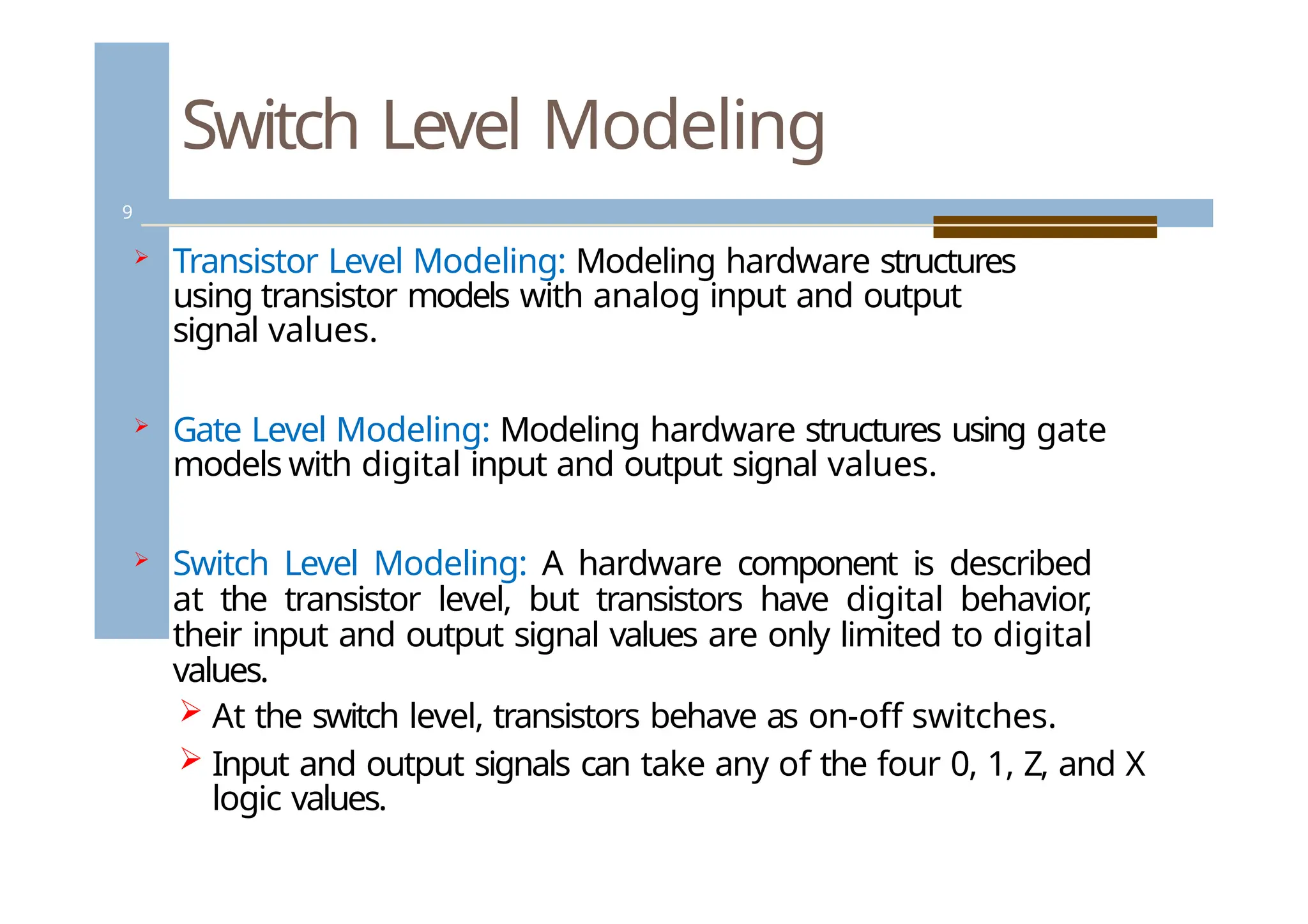
 Transistor Level Modeling: Modeling hardware structures
using transistor models with analog input and output
signal values.
 Gate Level Modeling: Modeling hardware structures using gate
models with digital input and output signal values.
 Switch Level Modeling: A hardware component is described
at the transistor level, but transistors have digital behavior
,
their input and output signal values are only limited to digital
values.
 At the switch level, transistors behave as on-off switches.
 Input and output signals can take any of the four 0, 1, Z, and X
logic values.

9. Switch Level Primitives
10
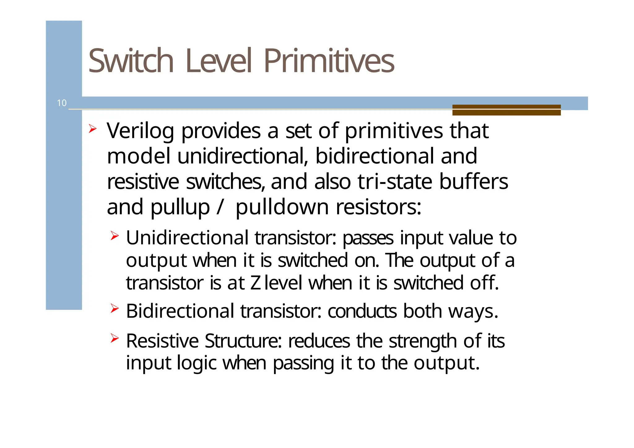
 Verilog provides a set of primitives that
model unidirectional, bidirectional and
resistive switches, and also tri-state buffers
and pullup / pulldown resistors:
 Unidirectional transistor: passes input value to
output when it is switched on. The output of a
transistor is at Zlevel when it is switched off.
 Bidirectional transistor: conducts both ways.
 Resistive Structure: reduces the strength of its
input logic when passing it to the output.

10. Switch level primitives
11

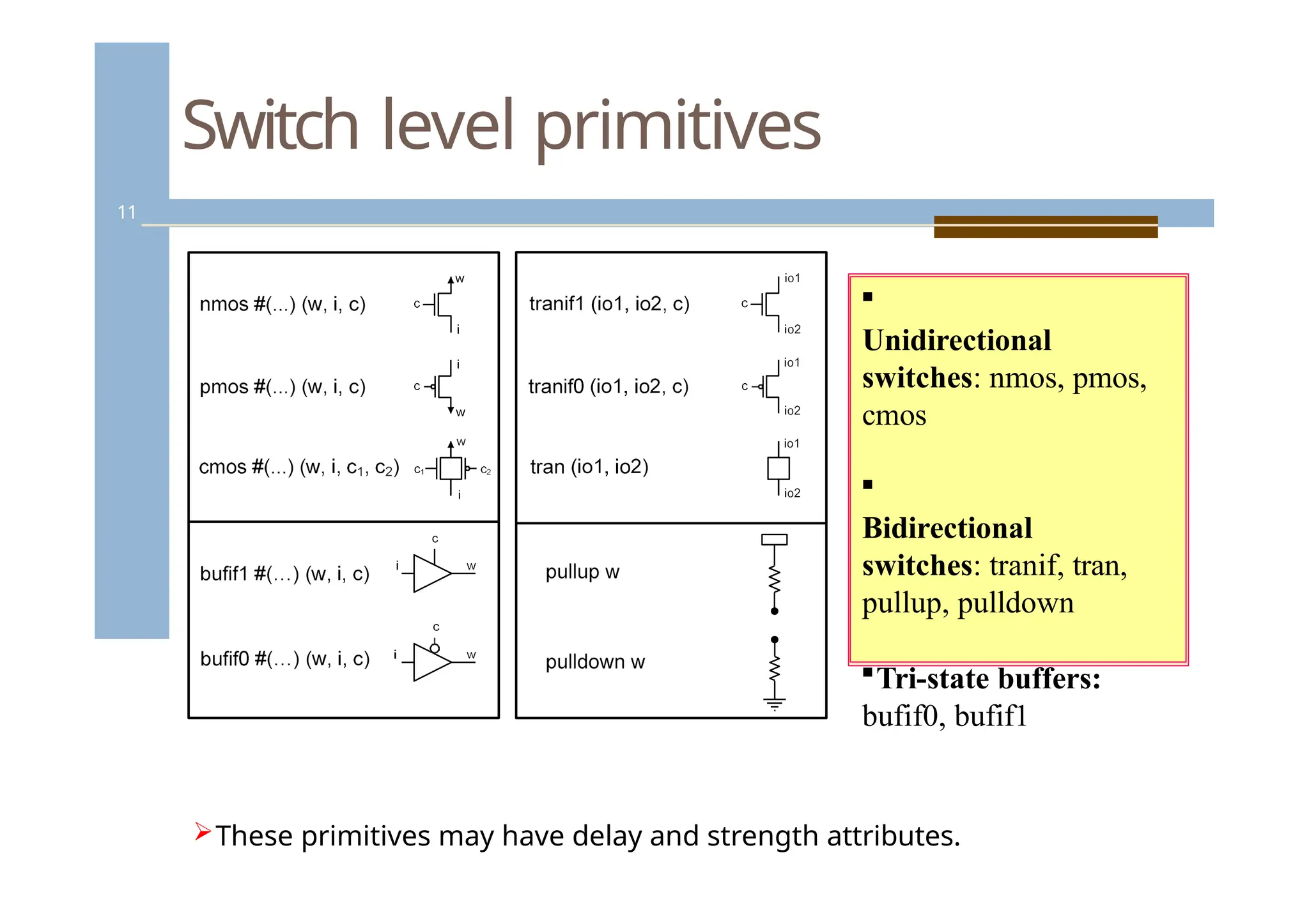
Unidirectional
switches: nmos, pmos,
cmos

Bidirectional
switches: tranif, tran,
pullup, pulldown
Tri-state buffers:
bufif0, bufif1
These primitives may have delay and strength attributes.

11. Switch Instantiation
12

12. 2-To-1 Multiplexer Using Pass Gates
13
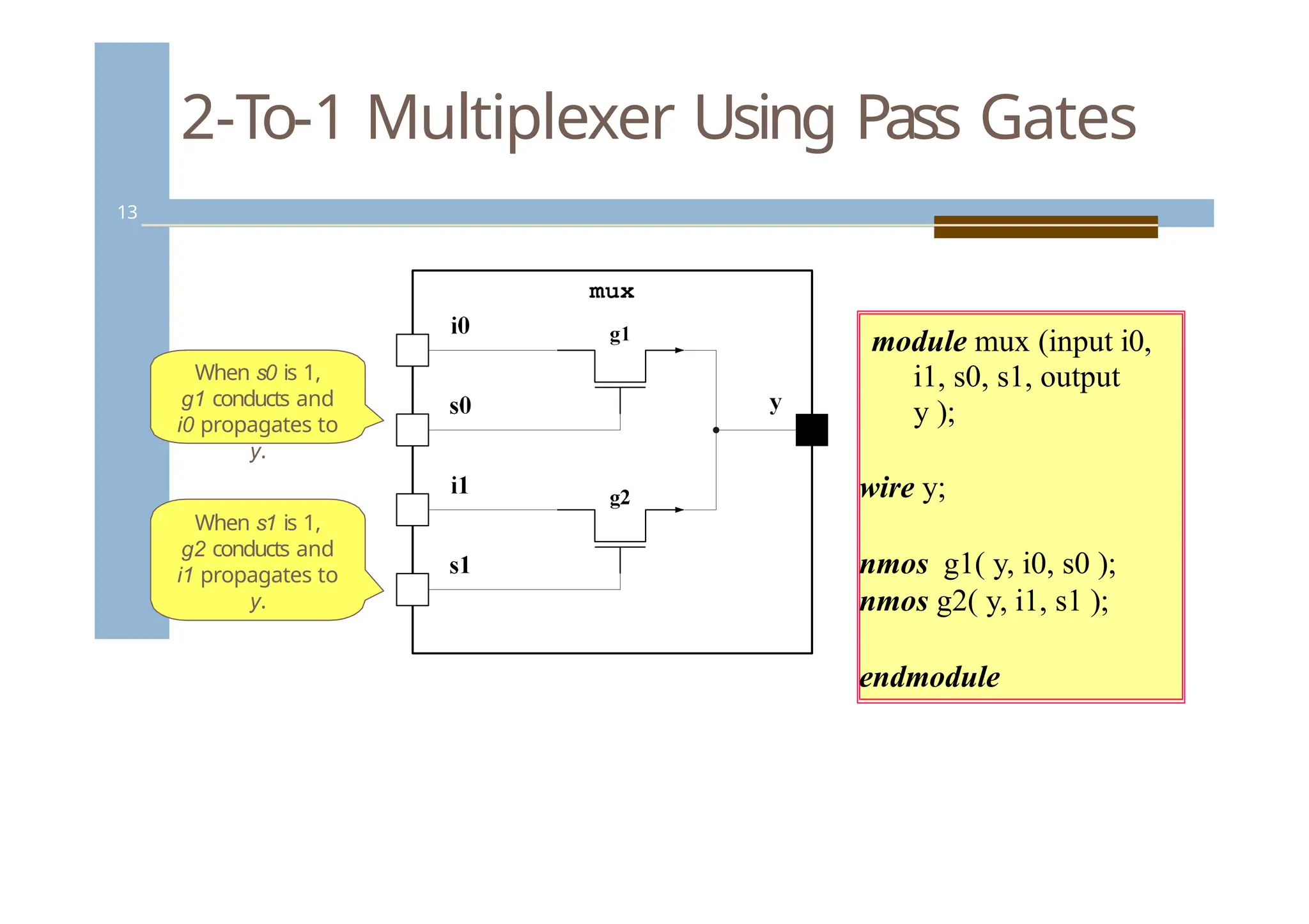
When s0 is 1,
g1 conducts and
i0 propagates to
y.
When s1 is 1,
g2 conducts and
i1 propagates to
y.
module mux (input i0,
i1, s0, s1, output
y );
wire y;
nmos g1( y, i0, s0 );
nmos g2( y, i1, s1 );
endmodule

13. Gate Level Modeling
14
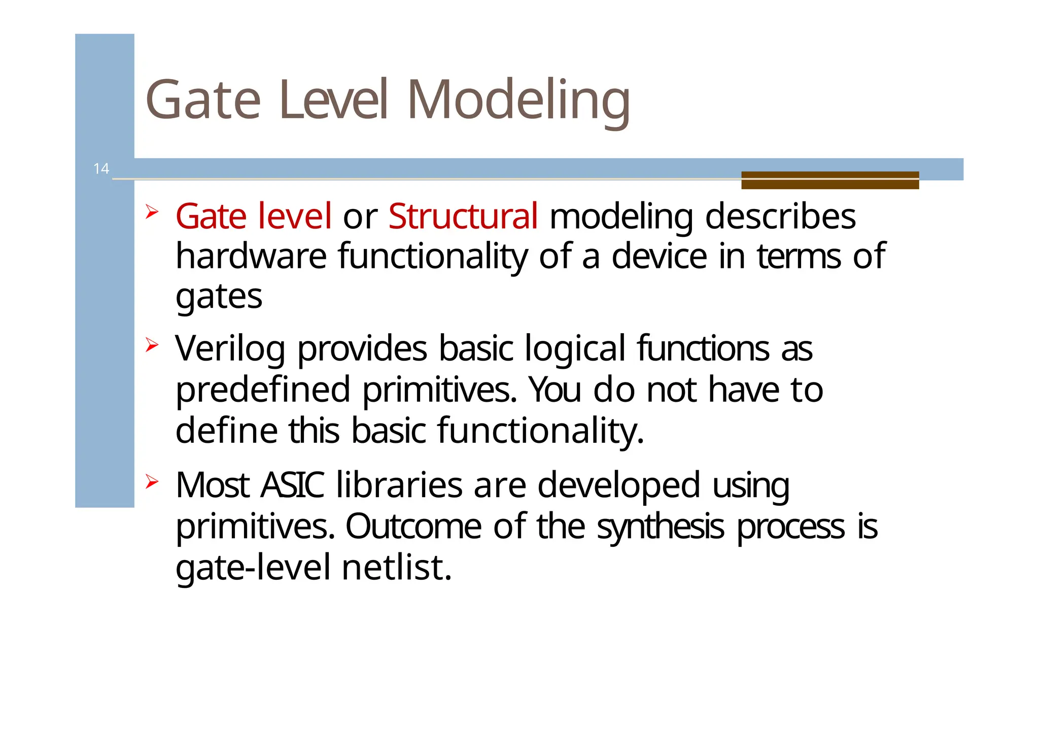
 Gate level or Structural modeling describes
hardware functionality of a device in terms of
gates
 Verilog provides basic logical functions as
predefined primitives. You do not have to
define this basic functionality.
 Most ASIC libraries are developed using
primitives. Outcome of the synthesis process is
gate-level netlist.

14. Built-in primitives
15
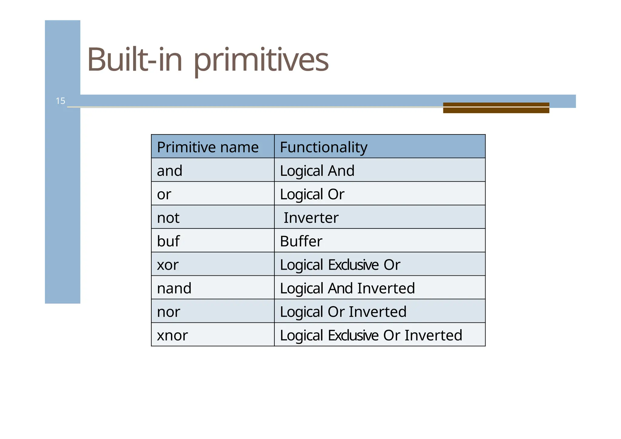
Primitive name Functionality
and Logical And
or Logical Or
not Inverter
buf Buffer
xor Logical Exclusive Or
nand Logical And Inverted
nor Logical Or Inverted
xnor Logical Exclusive Or Inverted

15. Gate Level Modeling
16
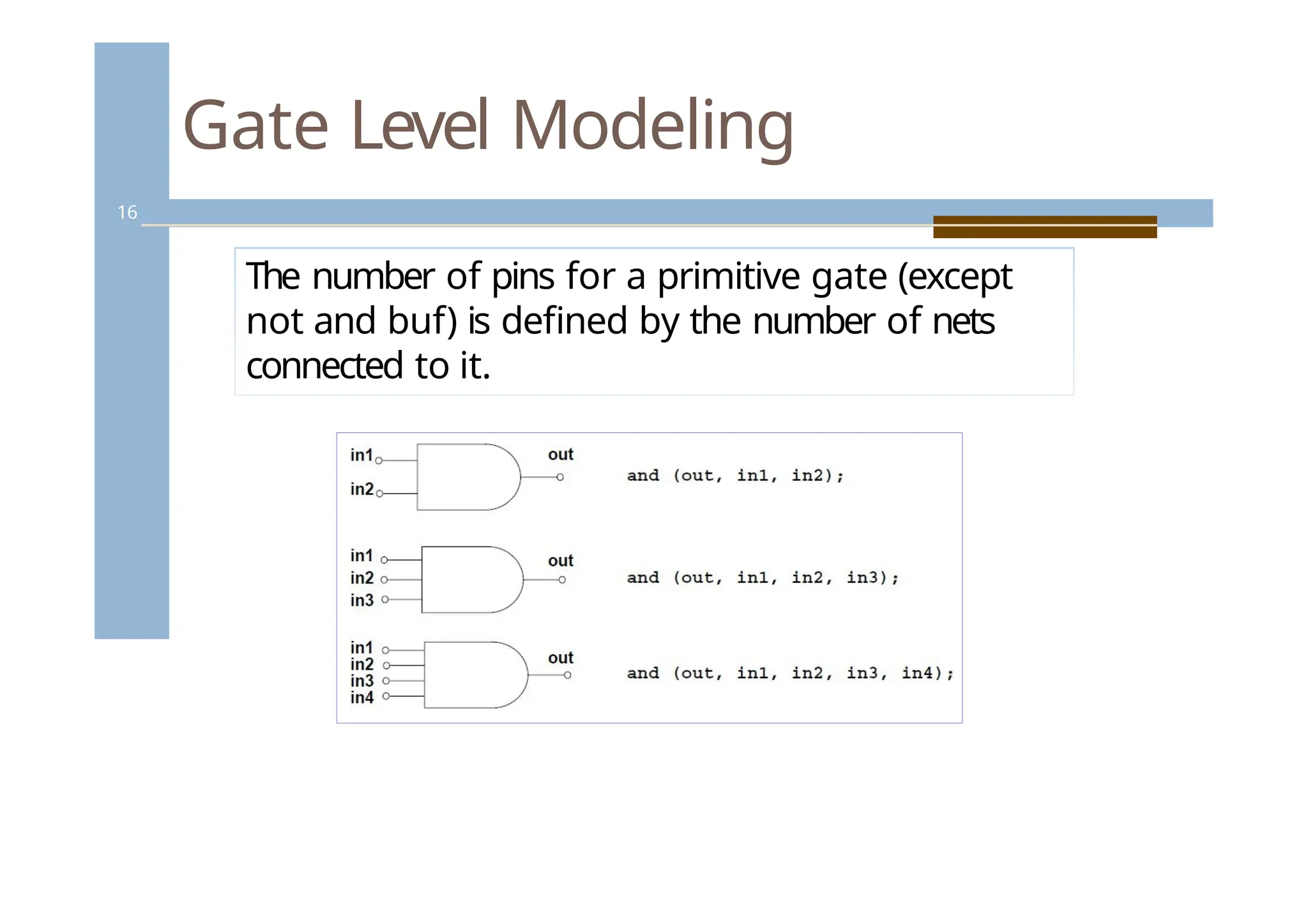
The number of pins for a primitive gate (except
not and buf) is defined by the number of nets
connected to it.

16. Gate Level Modeling - Primitive
Instantiation
17
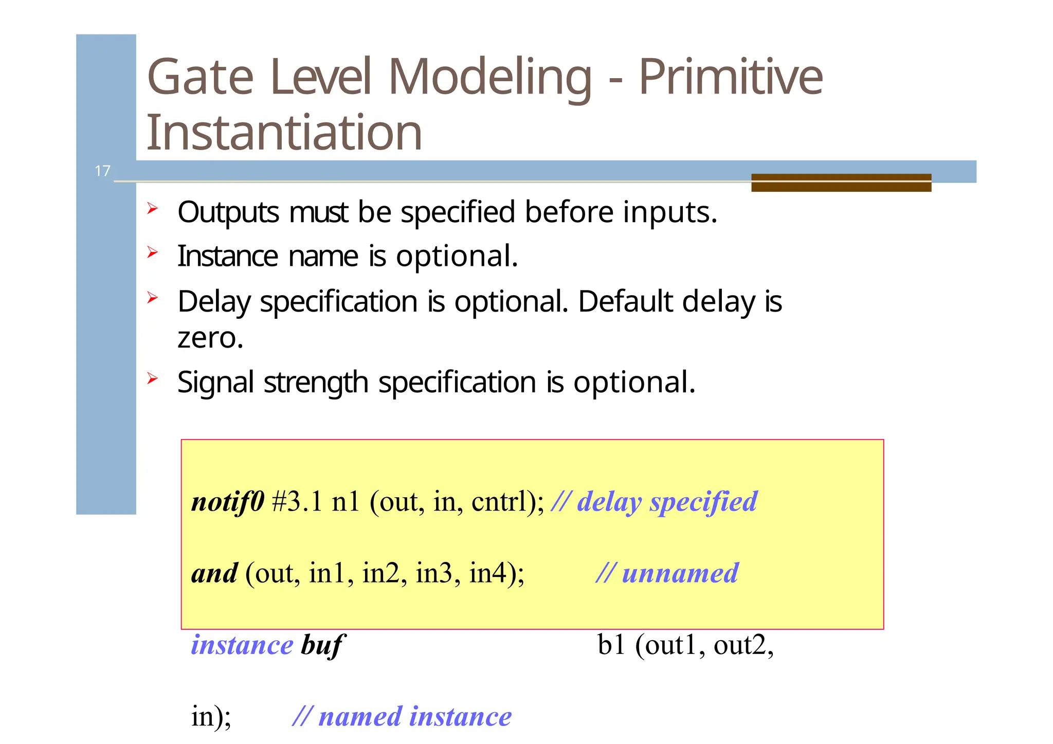
 Outputs must be specified before inputs.
 Instance name is optional.
 Delay specification is optional. Default delay is
zero.
 Signal strength specification is optional.
notif0 #3.1 n1 (out, in, cntrl); // delay specified
and (out, in1, in2, in3, in4); // unnamed
instance buf b1 (out1, out2,
in); // named instance

17. Gate Level Modeling –
delay specification
18
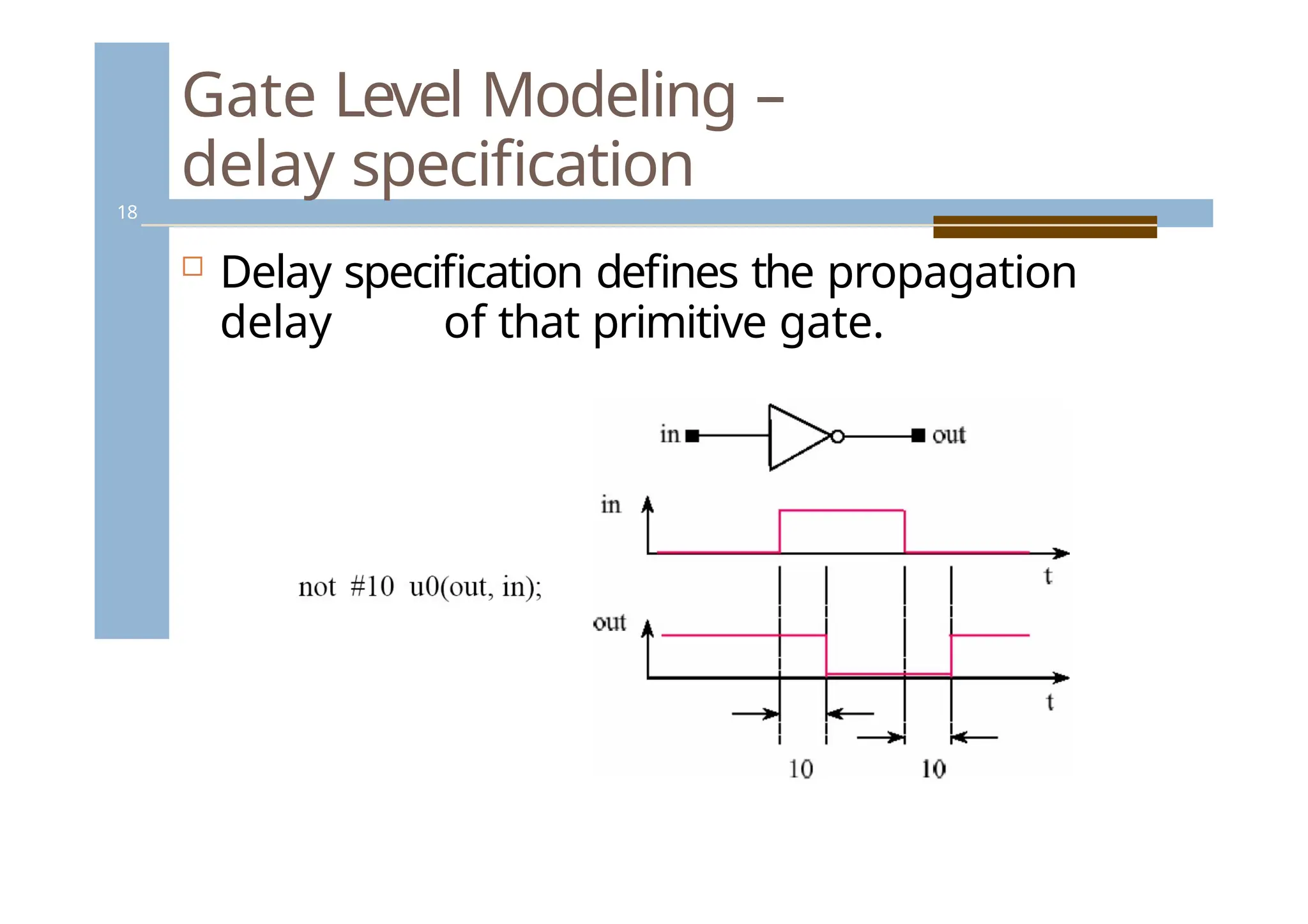
 Delay specification defines the propagation
delay of that primitive gate.

18. 3 2
Gate Level Modeling –
delay specification
19
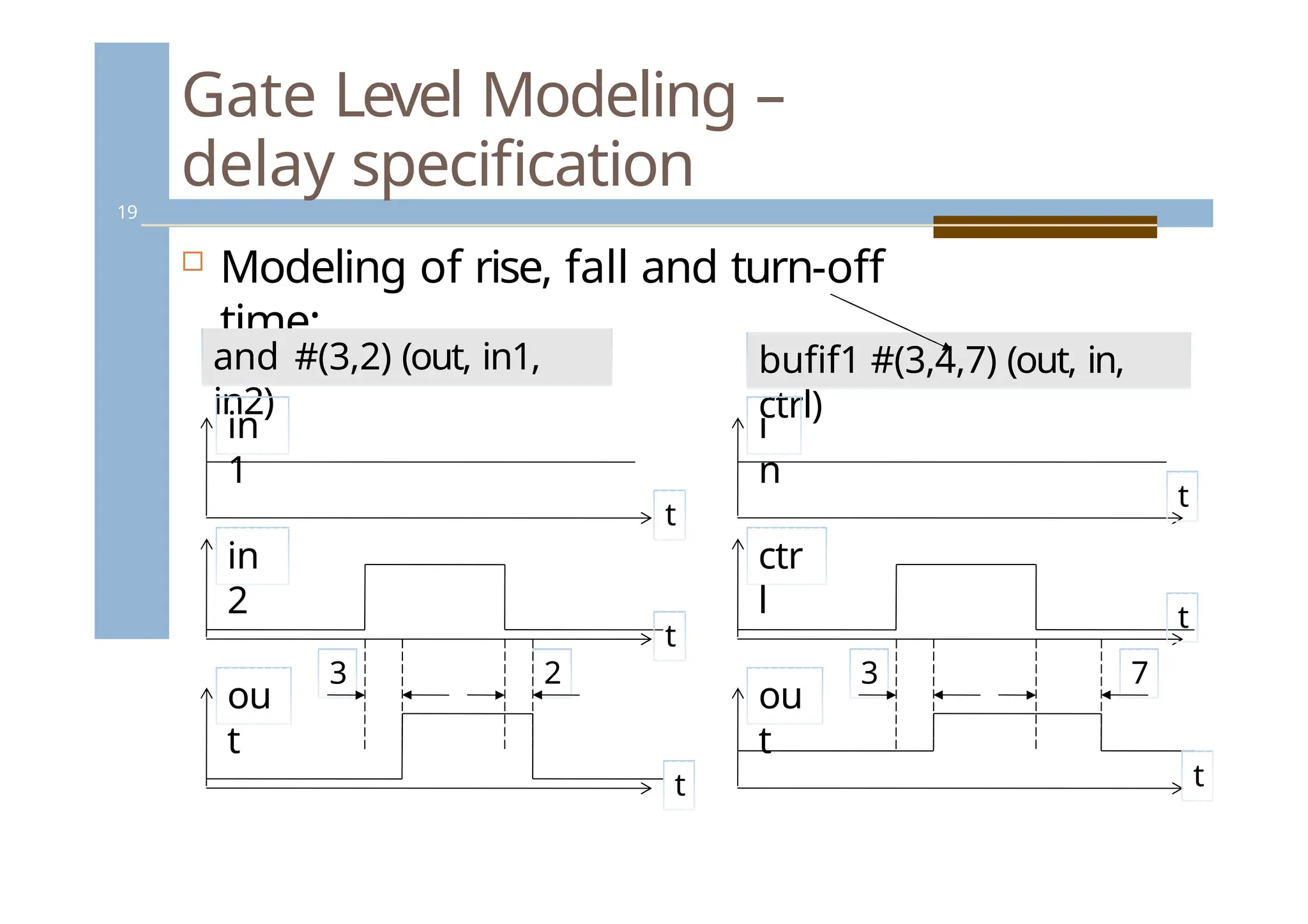
 Modeling of rise, fall and turn-off
time:
and #(3,2) (out, in1,
in2)
bufif1 #(3,4,7) (out, in,
ctrl)
in
1
in
2
ou
t
3 7
i
n
ctr
l
ou
t
t
t
t
t
t
t

19. User Defined Primitives
20
 UDPs permit the user to augment the set of
pre- defined primitive elements.
 Use of UDPs reduces the amount of
memory required for simulation.
 Both level-sensitive and edge-sensitive
behaviors are supported.

20. UDP Table Symbols
21

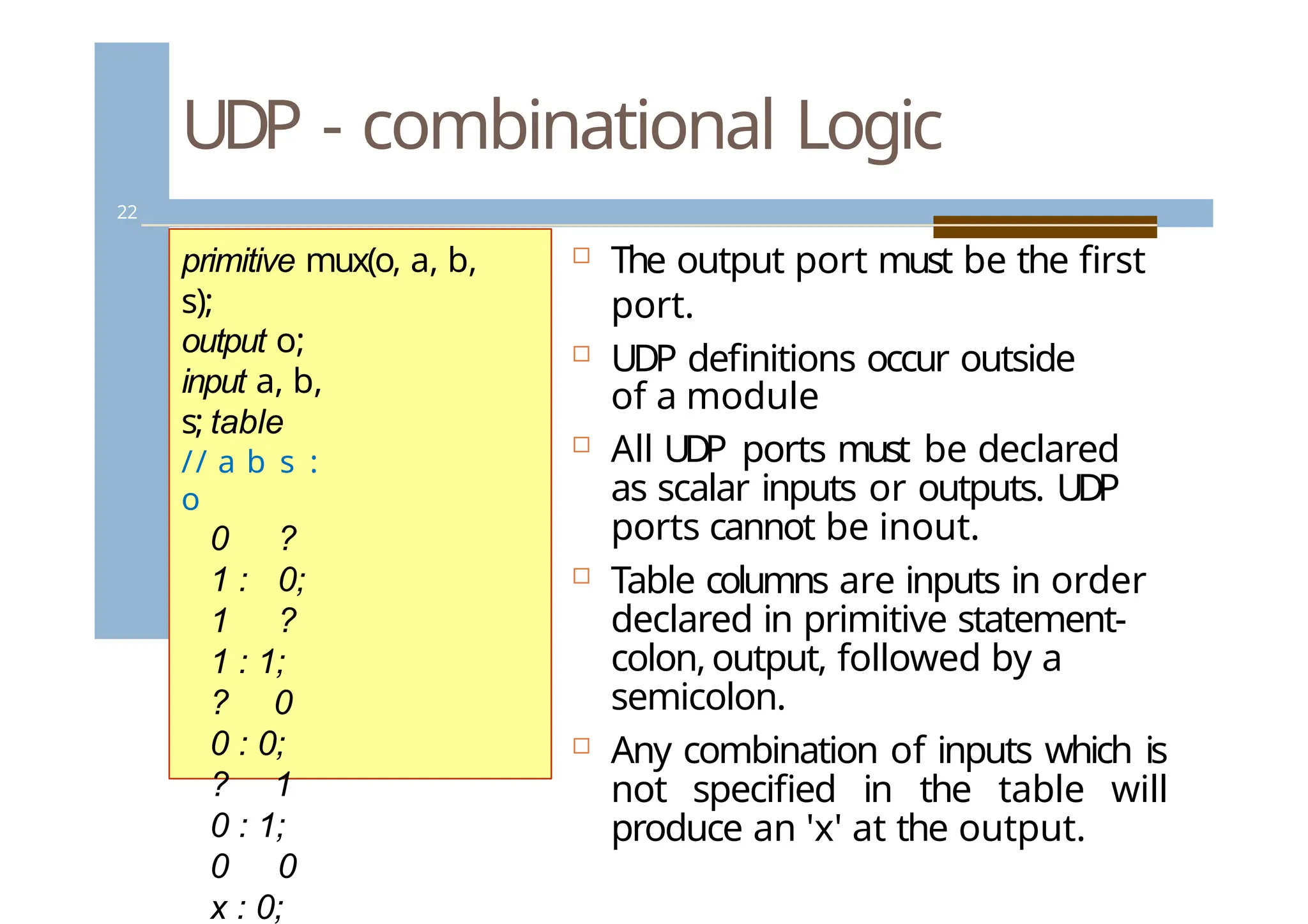
21. UDP - combinational Logic
22
 The output port must be the first
port.
 UDP definitions occur outside
of a module
 All UDP ports must be declared
as scalar inputs or outputs. UDP
ports cannot be inout.
 Table columns are inputs in order
declared in primitive statement-
colon,output, followed by a
semicolon.
 Any combination of inputs which is
not specified in the table will
produce an 'x' at the output.
primitive mux(o, a, b,
s);
output o;
input a, b,
s; table
// a b s :
o
0 ?
1 : 0;
1 ?
1 : 1;
? 0
0 : 0;
? 1
0 : 1;
0 0
x : 0;

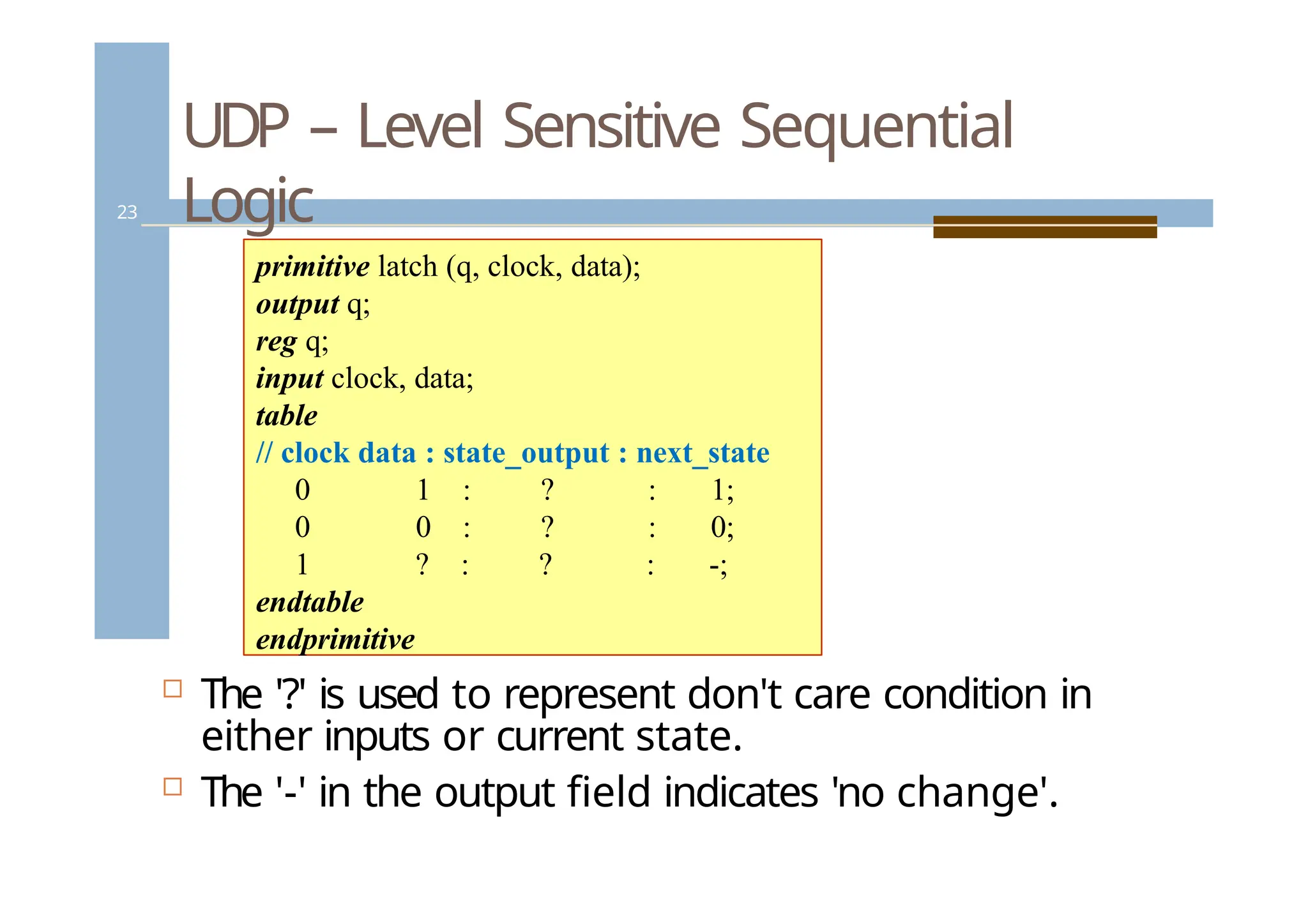
22. UDP – Level Sensitive Sequential
Logic
23
 The '?' is used to represent don't care condition in
either inputs or current state.
 The '-' in the output field indicates 'no change'.
primitive latch (q, clock, data);
output q;
reg q;
input clock, data;
table
// clock data : state_output : next_state
0 1 : ? : 1;
0 0 : ? : 0;
1 ? : ? : -;
endtable
endprimitive

23. UDP – Edge Sensitive Sequential
Logic
24
primitive d_edge_ff (q, clock, data);
output q;
reg q;
input clock, data;
table
// obtain output on rising edge of
clock
// clock data state next
(01) 0
:
? : 0;
(01) 1
:
? : 1;
(0x) 1
:
1 : 1;
(0x) 0
:
0 : 0;
// ignore negative edge of clock
(?0) ? : ? : -;
// ignore data changes on steady
clock
? (??) : ? : -;
endtable
endprimitive

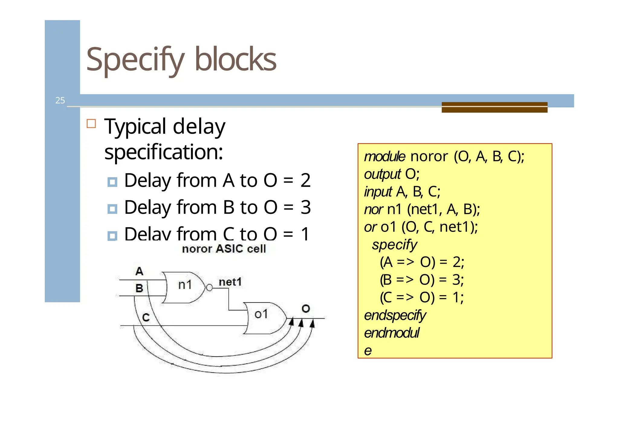
24. Specify blocks
25
 Typical delay
specification:
🞑 Delay from A to O = 2
🞑 Delay from B to O = 3
🞑 Delay from C to O = 1
module noror (O, A, B, C);
output O;
input A, B, C;
nor n1 (net1, A, B);
or o1 (O, C, net1);
specify
(A => O) = 2;
(B => O) = 3;
(C => O) = 1;
endspecify
endmodul
e

25. Specify blocks
26
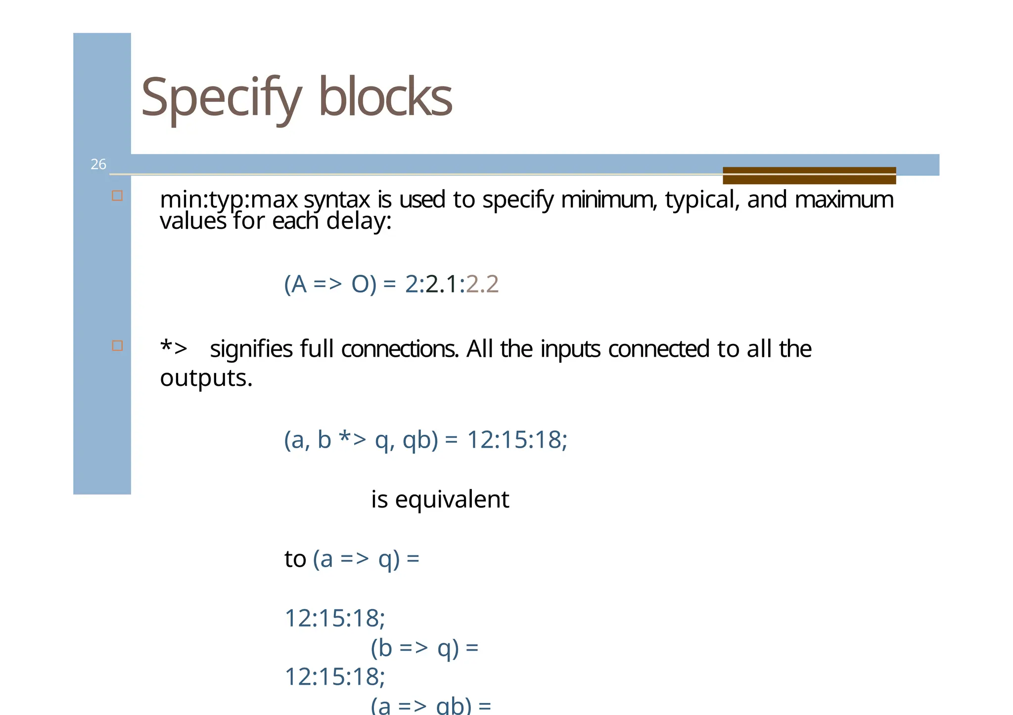
 min:typ:max syntax is used to specify minimum, typical, and maximum
values for each delay:
(A => O) = 2:2.1:2.2
 *> signifies full connections. All the inputs connected to all the
outputs.
(a, b *> q, qb) = 12:15:18;
is equivalent
to (a => q) =
12:15:18;
(b => q) =
12:15:18;
(a => qb) =

26. Parameters in specify blocks
27
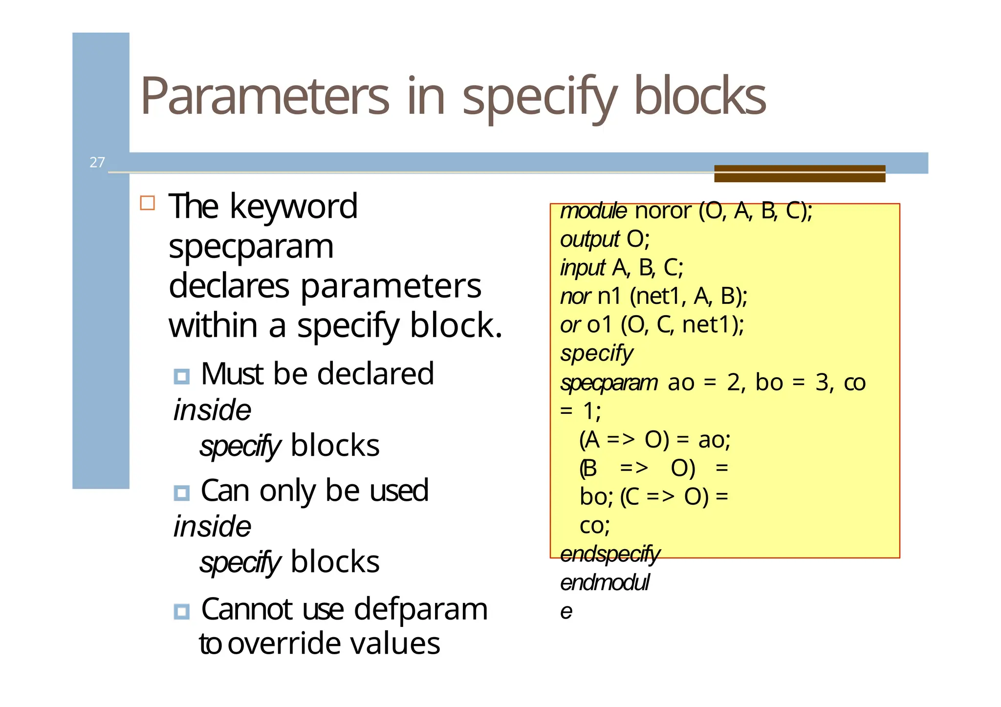
 The keyword
specparam
declares parameters
within a specify block.
🞑 Must be declared
inside
specify blocks
🞑 Can only be used
inside
specify blocks
🞑 Cannot use defparam
tooverride values
module noror (O, A, B, C);
output O;
input A, B, C;
nor n1 (net1, A, B);
or o1 (O, C, net1);
specify
specparam ao = 2, bo = 3, co
= 1;
(A => O) = ao;
(B => O) =
bo; (C => O) =
co;
endspecify
endmodul
e

27. Gate Level Modeling - Primitive
Instantiation
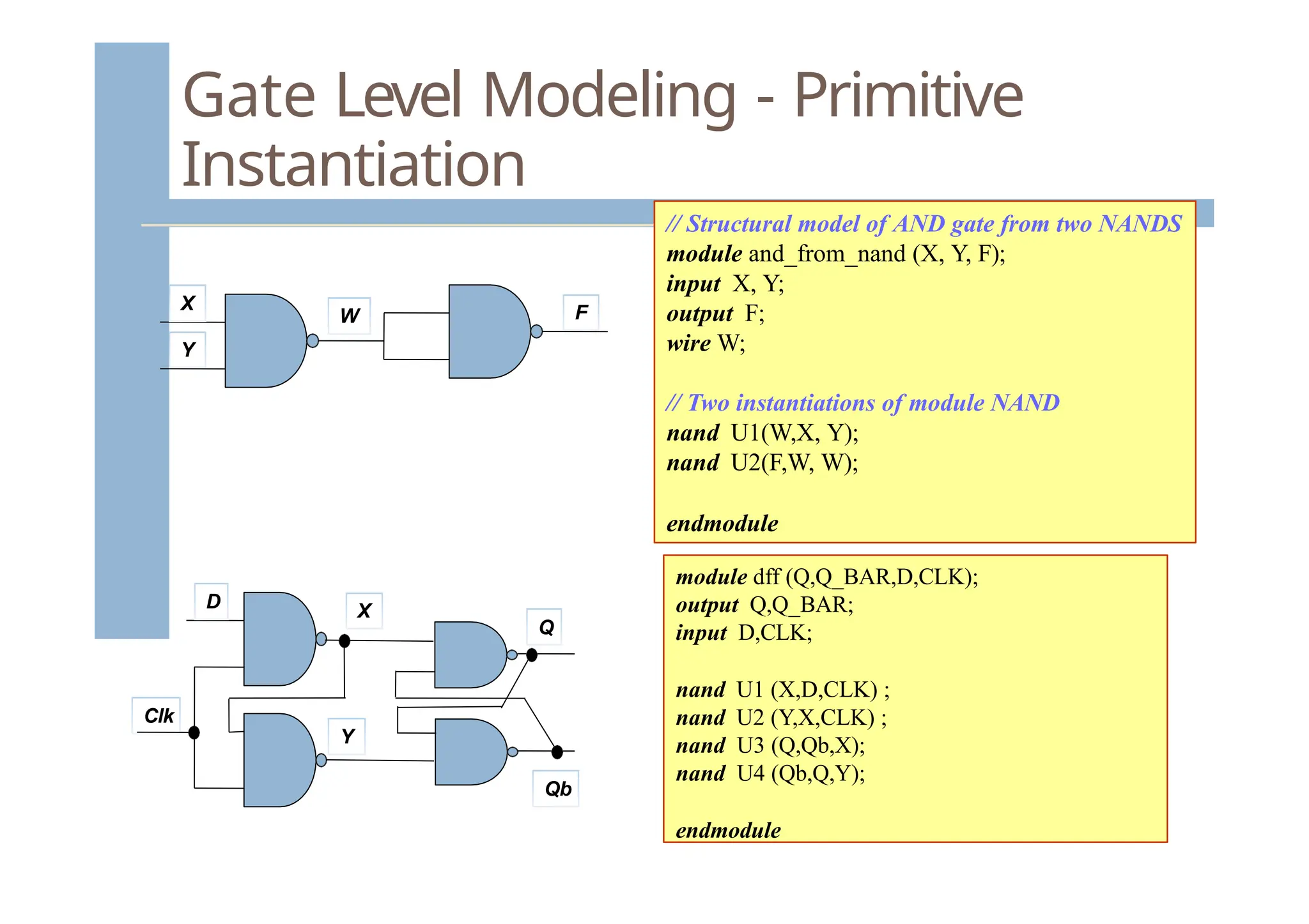
// Structural model of AND gate from two NANDS
module and_from_nand (X, Y, F);
input X, Y;
output F;
wire W;
// Two instantiations of module NAND
nand U1(W,X, Y);
nand U2(F,W, W);
endmodule
X
Y
W F
module dff (Q,Q_BAR,D,CLK);
output Q,Q_BAR;
input D,CLK;
nand U1 (X,D,CLK) ;
nand U2 (Y,X,CLK) ;
nand U3 (Q,Qb,X);
nand U4 (Qb,Q,Y);
endmodule
D
Clk
Q
Qb
X
Y

28. Strength modeling
29
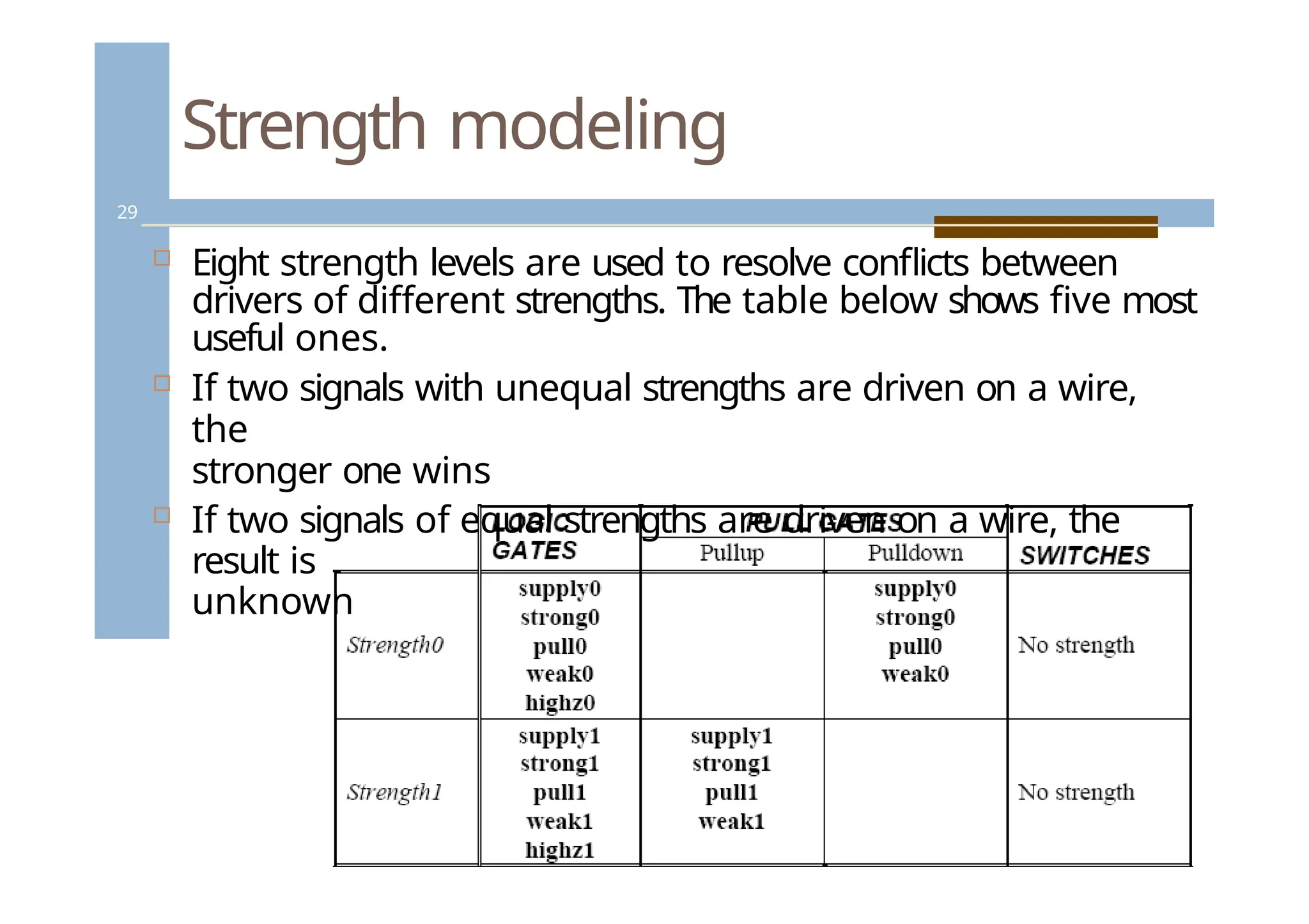
 Eight strength levels are used to resolve conflicts between
drivers of different strengths. The table below shows five most
useful ones.
 If two signals with unequal strengths are driven on a wire,
the
stronger one wins
 If two signals of equal strengths are driven on a wire, the
result is
unknown

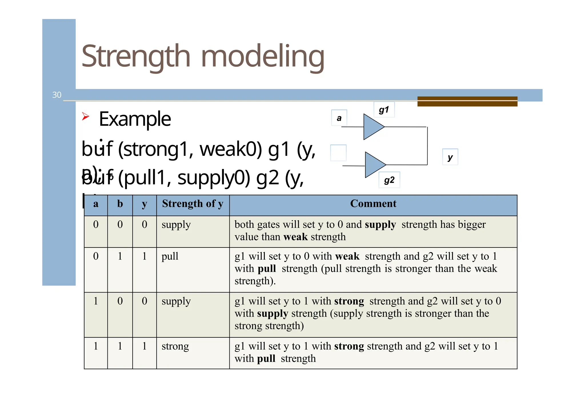
29. Strength modeling
30
 Example
:
buf (pull1, supply0) g2 (y,
b);
a b y Strength of y Comment
0 0 0 supply both gates will set y to 0 and supply strength has bigger
value than weak strength
0 1 1 pull g1 will set y to 0 with weak strength and g2 will set y to 1
with pull strength (pull strength is stronger than the weak
strength).
1 0 0 supply g1 will set y to 1 with strong strength and g2 will set y to 0
with supply strength (supply strength is stronger than the
strong strength)
1 1 1 strong g1 will set y to 1 with strong strength and g2 will set y to 1
with pull strength
a
buf (strong1, weak0) g1 (y,
a); b
g1
g2
y

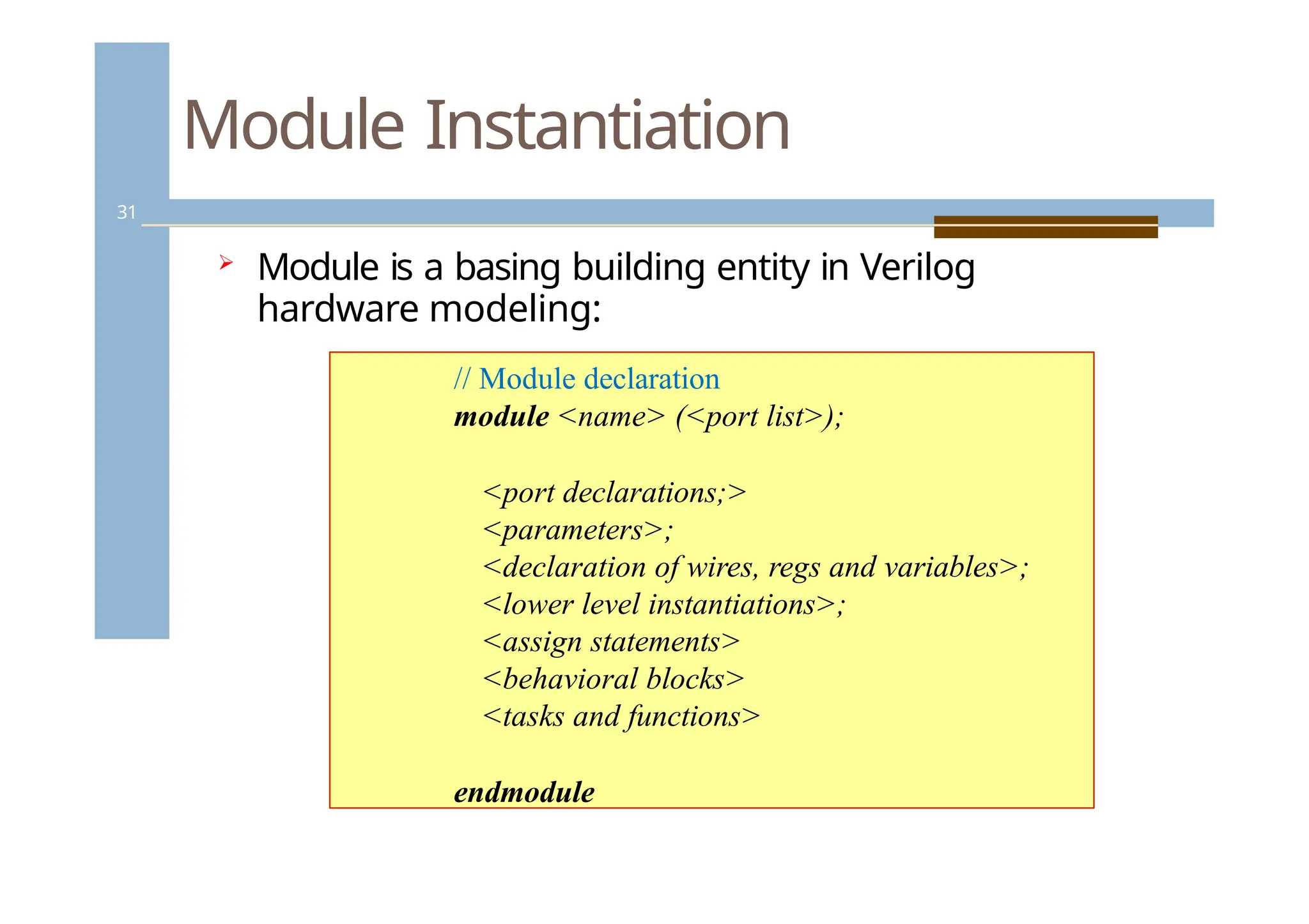
30. Module Instantiation
31
 Module is a basing building entity in Verilog
hardware modeling:
// Module declaration
module <name> (<port list>);
<port declarations;>
<parameters>;
<declaration of wires, regs and variables>;
<lower level instantiations>;
<assign statements>
<behavioral blocks>
<tasks and functions>
endmodule

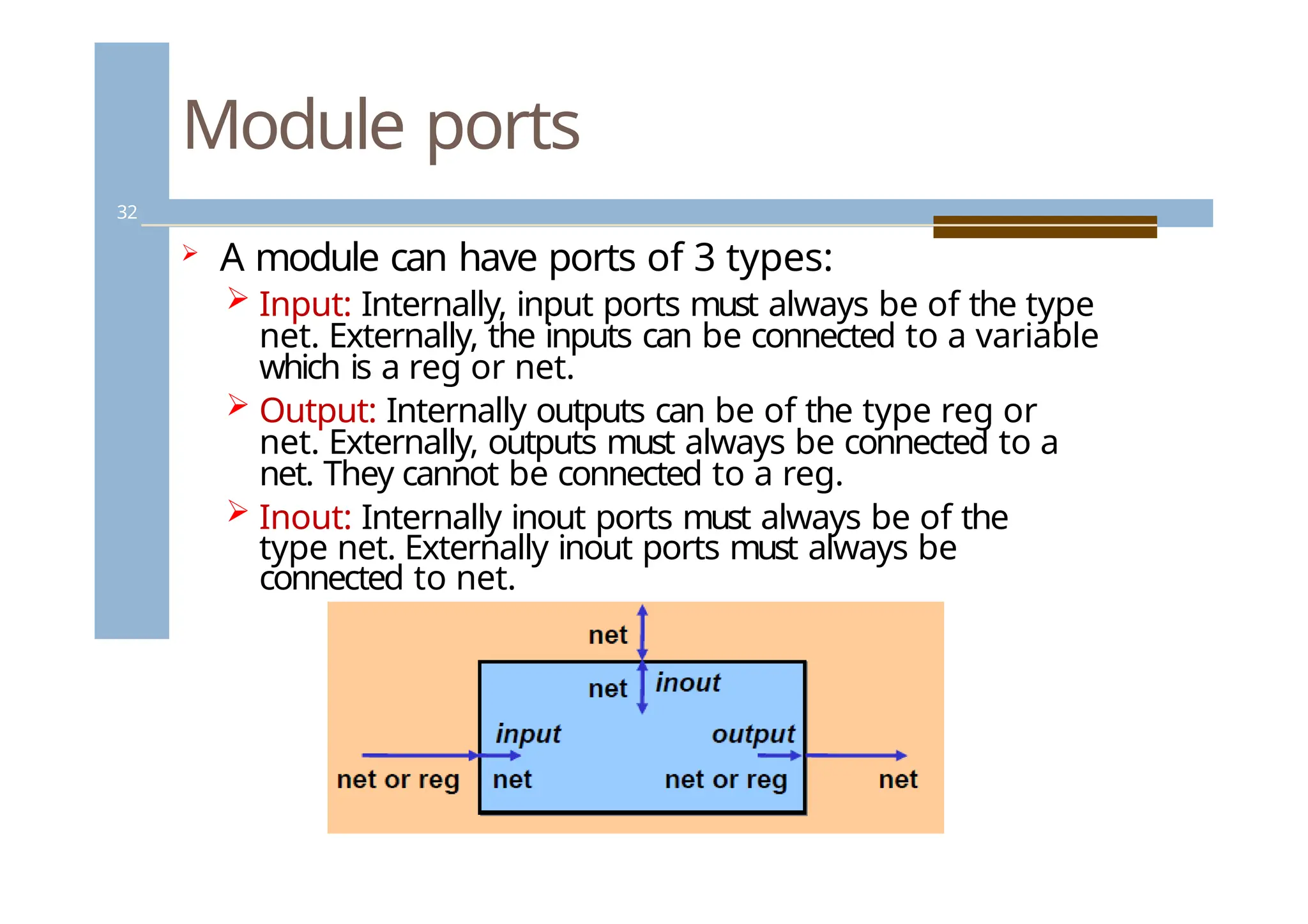
31. Module ports
32
 A module can have ports of 3 types:
 Input: Internally, input ports must always be of the type
net. Externally, the inputs can be connected to a variable
which is a reg or net.
 Output: Internally outputs can be of the type reg or
net. Externally, outputs must always be connected to a
net. They cannot be connected to a reg.
 Inout: Internally inout ports must always be of the
type net. Externally inout ports must always be
connected to net.

32. Module ports
33
 Width matching: it is legal to connect internal
and external items of different sizes when
making inter- module port connections.
Warning will be issued when the width differs.
 Verilog allows ports to remain unconnected,
though this should be avoided. In particular,
inputs should never be left floating.

33. Module Instantiation
34
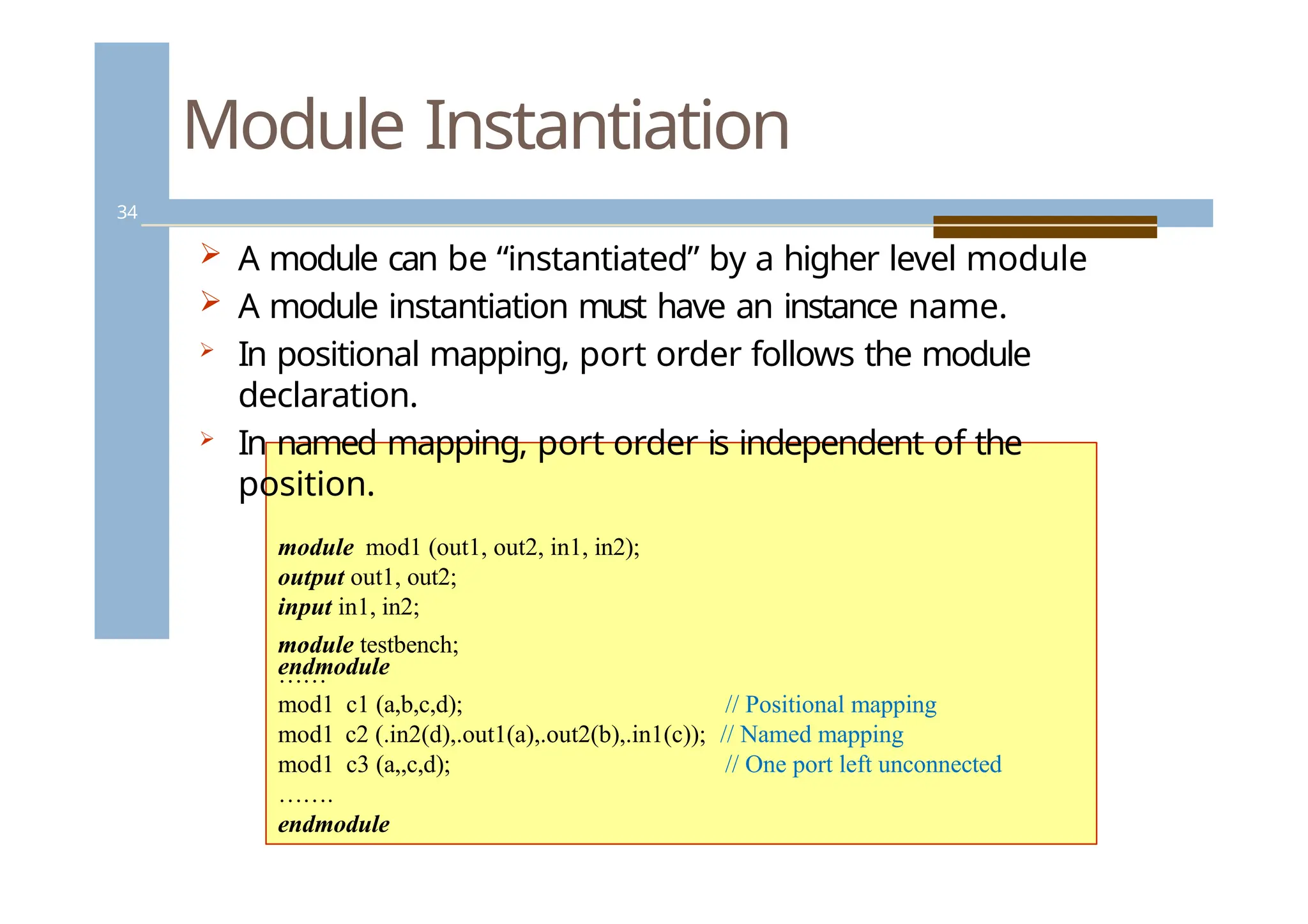
 A module can be “instantiated” by a higher level module
 A module instantiation must have an instance name.
 In positional mapping, port order follows the module
declaration.
 In named mapping, port order is independent of the
position.
module mod1 (out1, out2, in1, in2);
output out1, out2;
input in1, in2;
. . .
endmodule
module testbench;
……
mod1 c1 (a,b,c,d); // Positional mapping
mod1 c2 (.in2(d),.out1(a),.out2(b),.in1(c)); // Named mapping
mod1 c3 (a,,c,d); // One port left unconnected
…….
endmodule

34. Behavioural Modelling
35
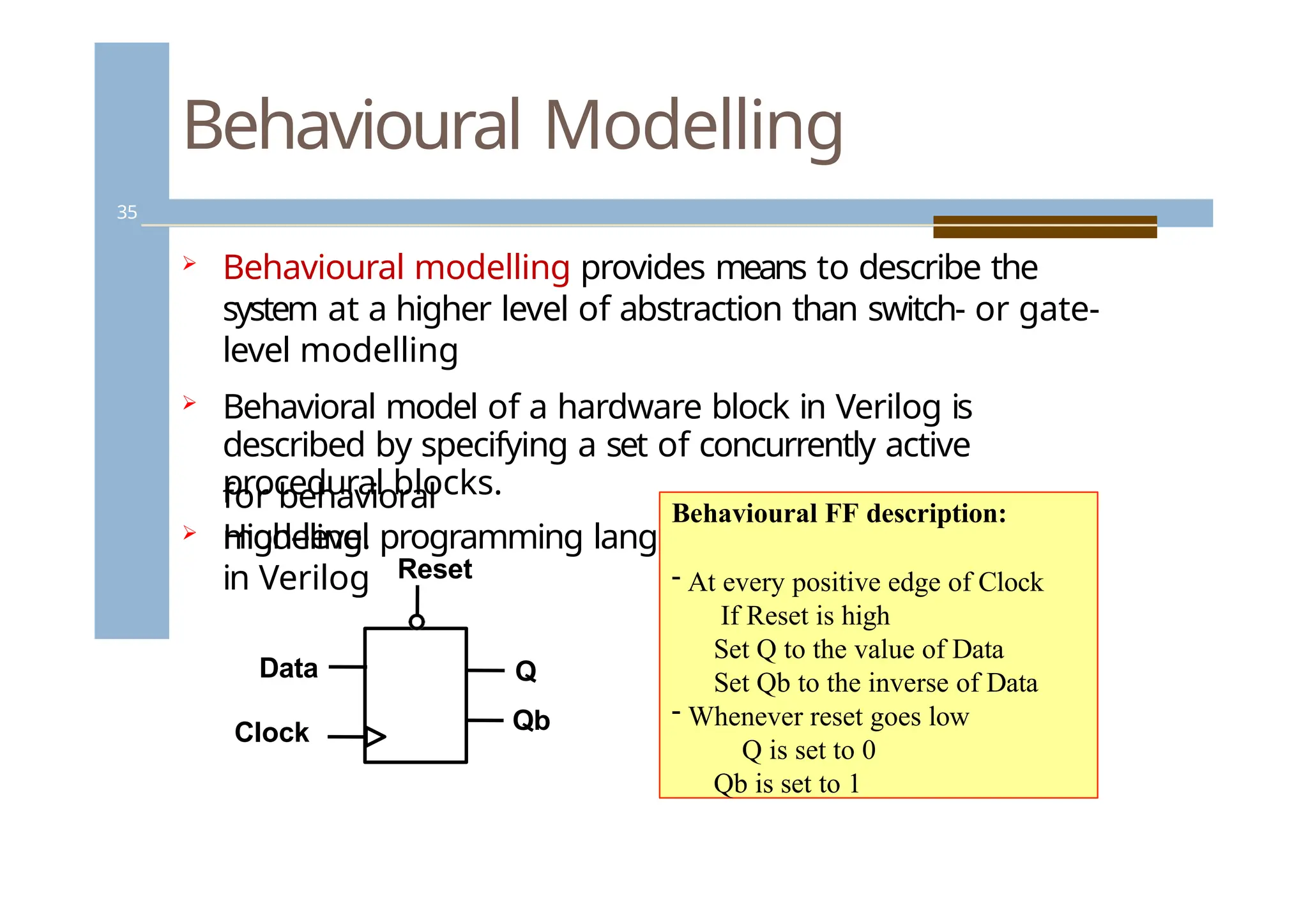
 Behavioural modelling provides means to describe the
system at a higher level of abstraction than switch- or gate-
level modelling
 Behavioral model of a hardware block in Verilog is
described by specifying a set of concurrently active
procedural blocks.
 High-level programming language constructs are available
in Verilog
for behavioral
modeling.
Reset
Clock
Q
Qb
Data
Behavioural FF description:
- At every positive edge of Clock
If Reset is high
Set Q to the value of Data
Set Qb to the inverse of Data
- Whenever reset goes low
Q is set to 0
Qb is set to 1

35. Register transfer level (RTL)
level
36
 The register transfer level, RTL, is a design level of
abstraction. “RTL” refers to coding that uses a subset
of the Verilog language.
 RTL is the level of abstraction below behavioral and
above
structural.
 Events are defined in terms of clocks and certain
behavioral constructs are not used.
 Some of Verilog constructs are not understood by
synthesizers. Each tool is different in the subset of the
language that it supports, but as time progresses the
differences become smaller.
 The simplest definition of what is RTL is “any code
that is synthesizable”.

36. Assignments
37
 Assignment is the basic mechanism for getting
values into nets and registers.
An assignment consists of two parts, a left-
hand side (LHS) and a right-hand
side (RHS), separated by the
equal sign (=).
 The right-hand side can be any expression
that evaluates to a value.
 The left-hand side indicates the variable
that the right-hand side is to be assigned
to.
 Assignments can be either continuous or
procedural

37. Assignments
38
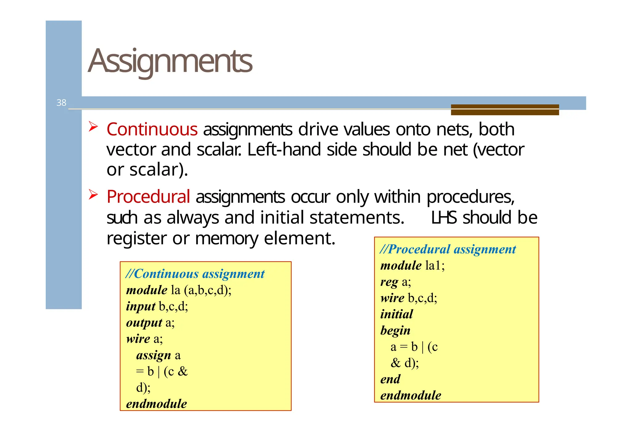
 Continuous assignments drive values onto nets, both
vector and scalar
. Left-hand side should be net (vector
or scalar).
 Procedural assignments occur only within procedures,
such as always and initial statements. LHS should be
register or memory element.
//Continuous assignment
module la (a,b,c,d);
input b,c,d;
output a;
wire a;
assign a
= b | (c &
d);
endmodule
//Procedural assignment
module la1;
reg a;
wire b,c,d;
initial
begin
a = b | (c
& d);
end
endmodule

38. Continuous Assignments
39
 Combinational logic can be modeled with
continuous assignments, instead of using gates and
interconnect nets.
 Continuous assignments can be either explicit or
implicit.
 Syntax for an explicit continuous assignment:
<assign> [#delay] [strength] <net_name> =
<expression>

39. Continuous Assignments
40
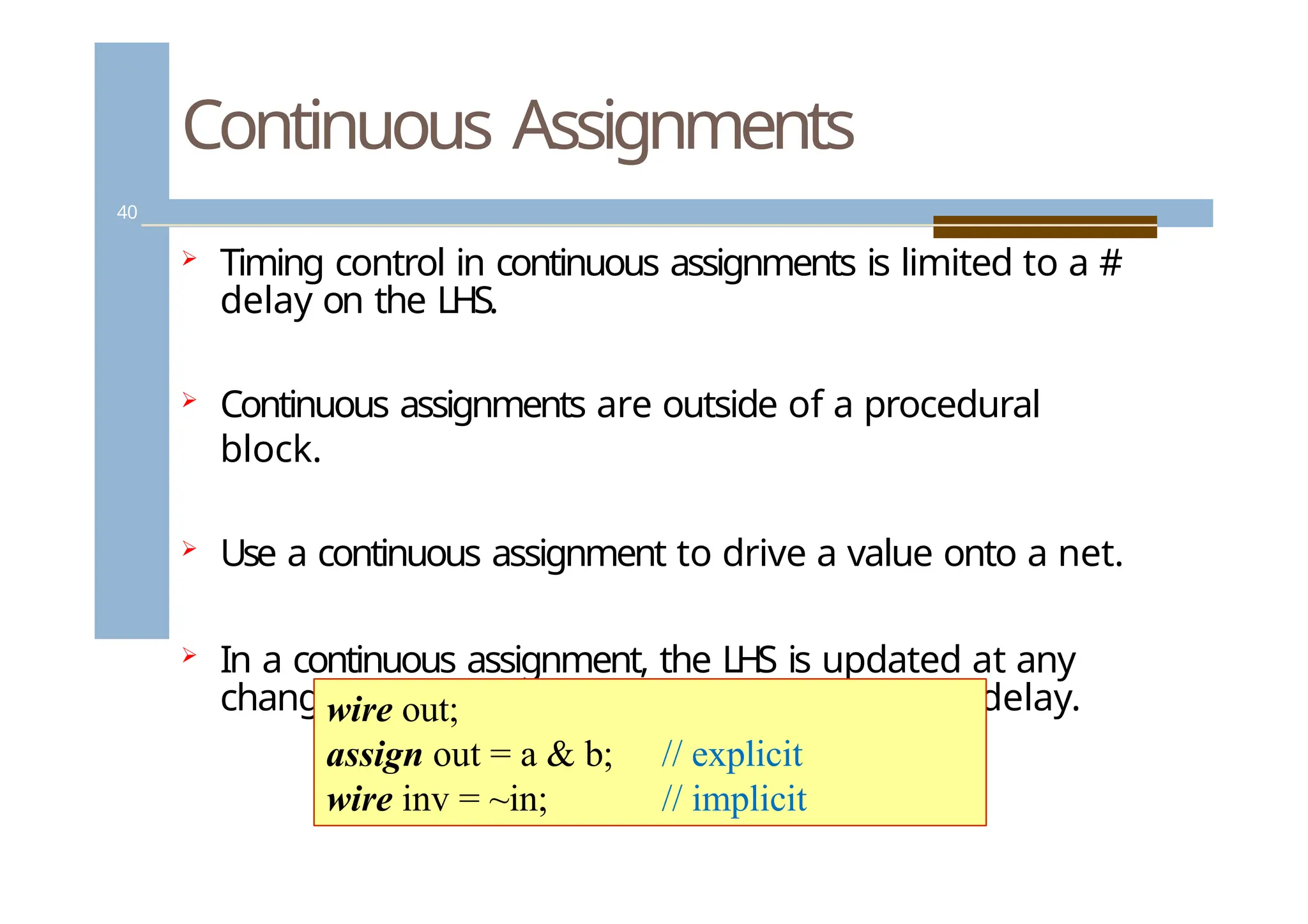
 Timing control in continuous assignments is limited to a #
delay on the LHS.
 Continuous assignments are outside of a procedural
block.
 Use a continuous assignment to drive a value onto a net.
 In a continuous assignment, the LHS is updated at any
change in the RHS expression, after a specified delay.
wire out;
assign out = a & b;
wire inv = ~in;
// explicit
// implicit

40. Procedural assignments
41
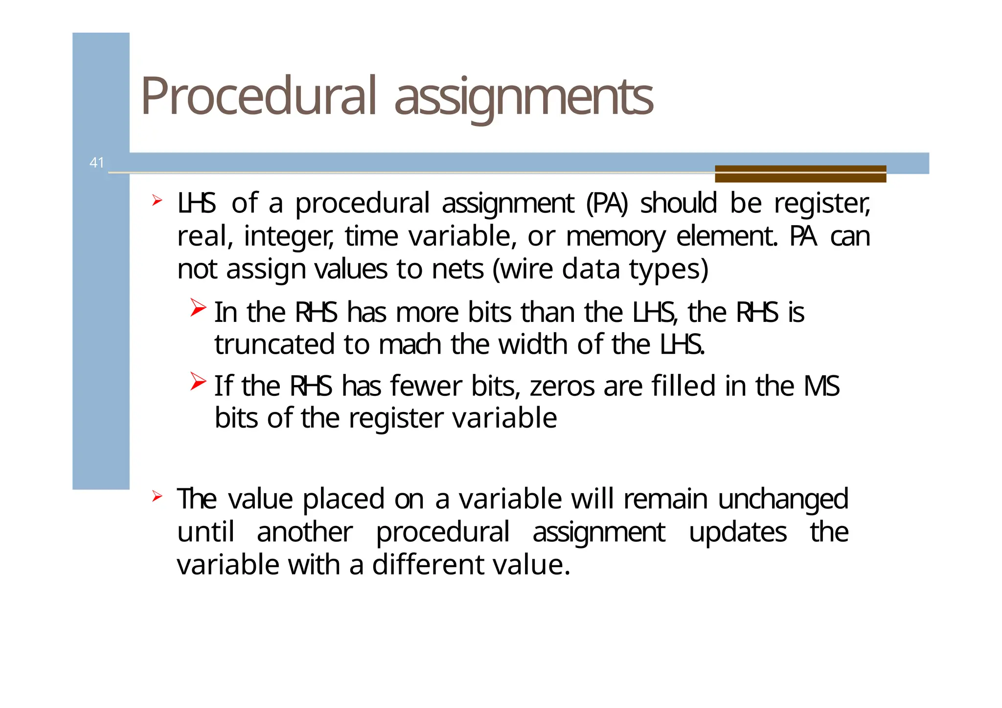
 LH
S of a procedural assignment (PA) should be register,
real, integer
, time variable, or memory element. P
A can
not assign values to nets (wire data types)
 In the RHS has more bits than the LHS, the RHS is
truncated to mach the width of the LHS.
 If the RHS has fewer bits, zeros are filled in the MS
bits of the register variable
 The value placed on a variable will remain unchanged
until another procedural assignment updates the
variable with a different value.

41. Procedural blocks
42
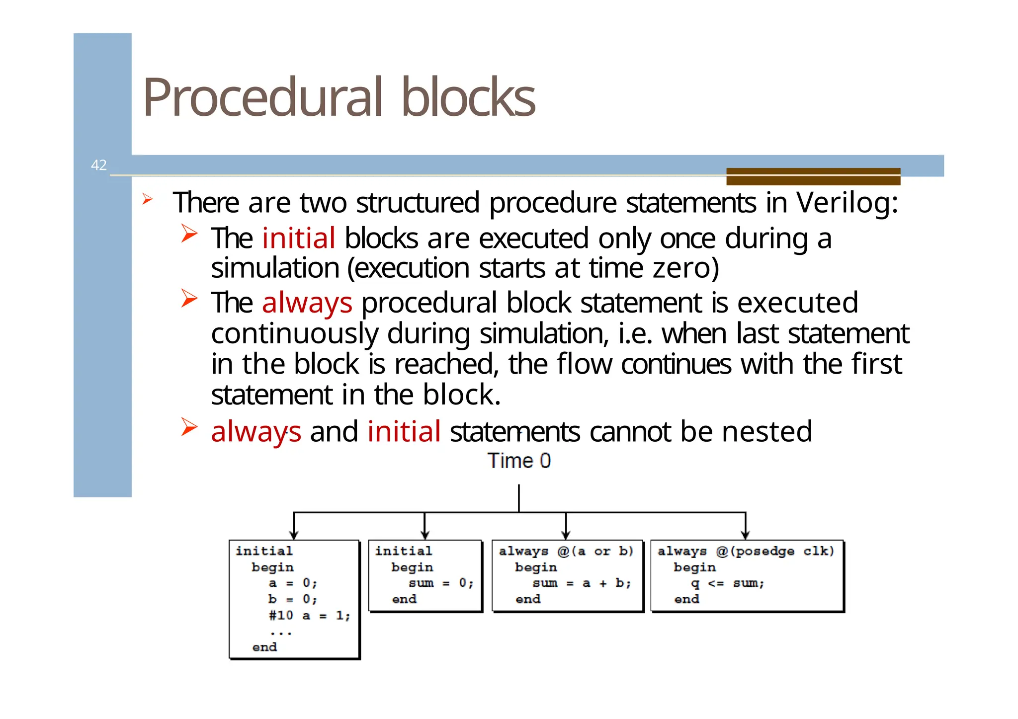
 There are two structured procedure statements in Verilog:
 The initial blocks are executed only once during a
simulation (execution starts at time zero)
 The always procedural block statement is executed
continuously during simulation, i.e. when last statement
in the block is reached, the flow continues with the first
statement in the block.
 always and initial statements cannot be nested

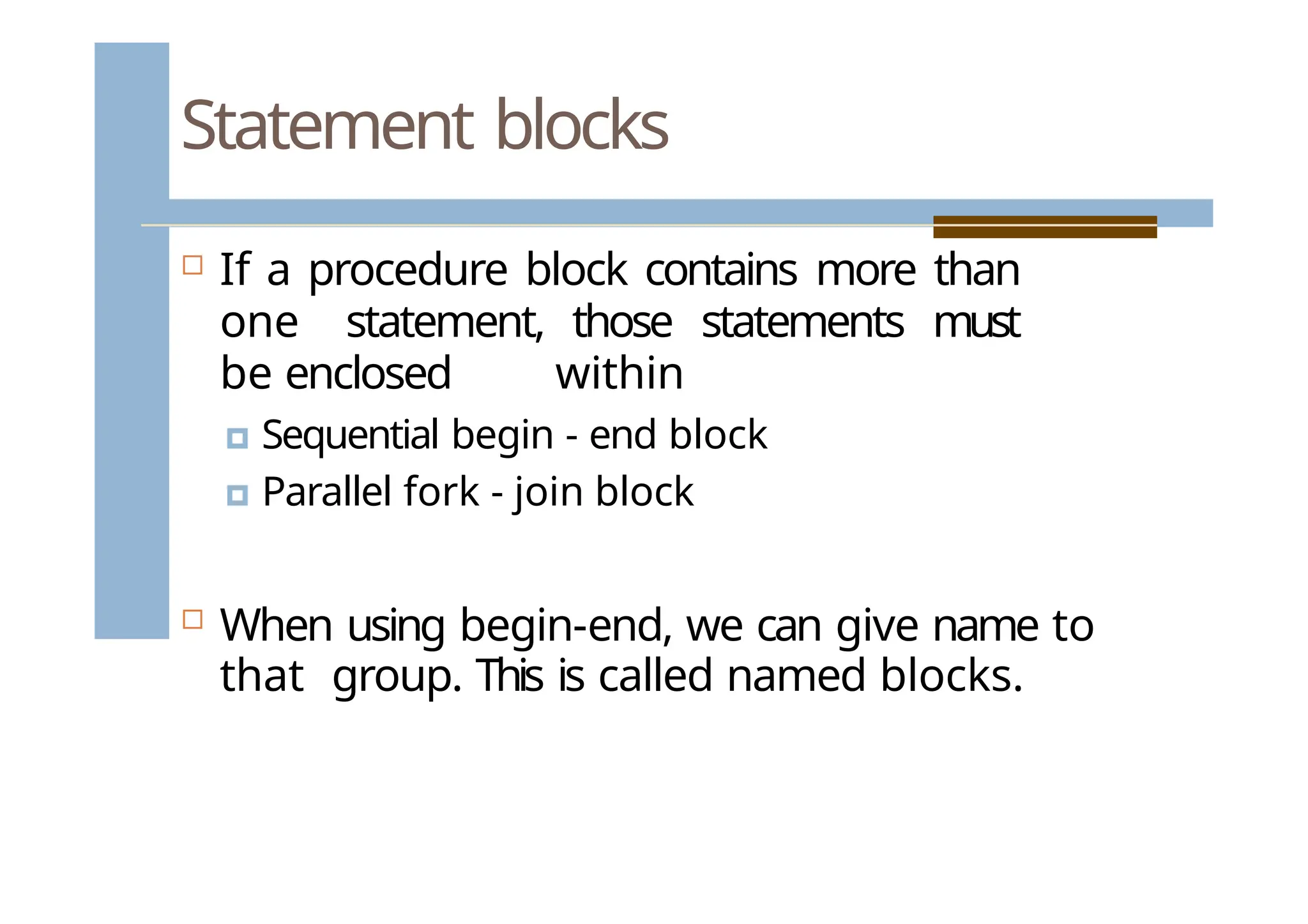
42. Statement blocks
 If a procedure block contains more than
one statement, those statements must
be enclosed within
🞑 Sequential begin - end block
🞑 Parallel fork - join block
 When using begin-end, we can give name to
that group. This is called named blocks.

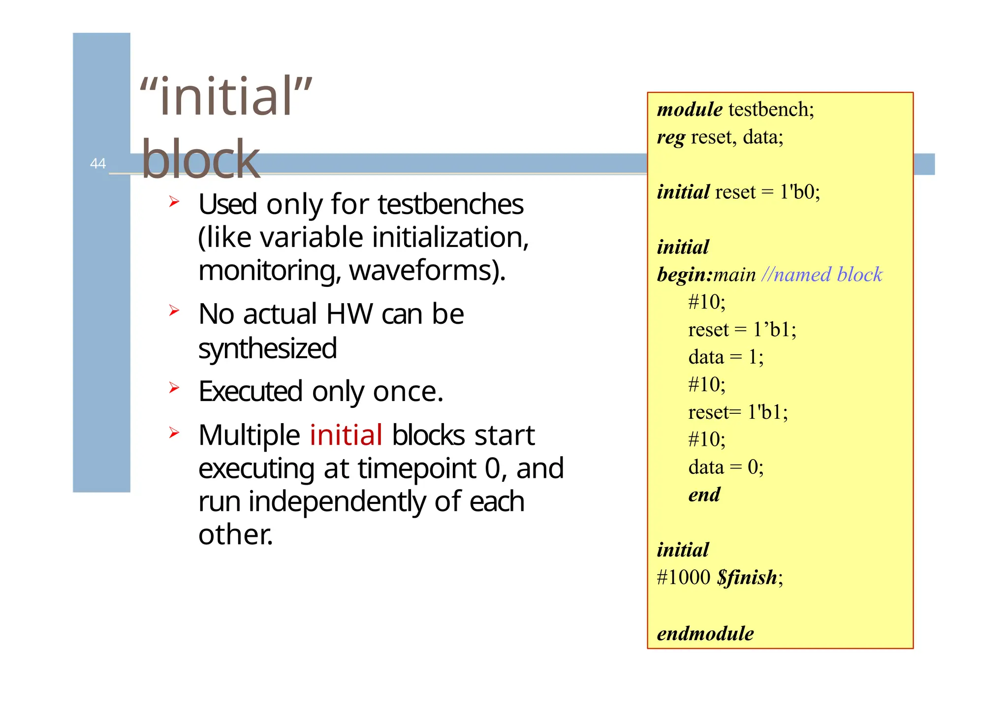
43. “initial”
block
44
 Used only for testbenches
(like variable initialization,
monitoring, waveforms).
 No actual HW can be
synthesized
 Executed only once.
 Multiple initial blocks start
executing at timepoint 0, and
run independently of each
other.
module testbench;
reg reset, data;
initial reset = 1'b0;
initial
begin:main //named block
#10;
reset = 1’b1;
data = 1;
#10;
reset= 1'b1;
#10;
data = 0;
end
initial
#1000 $finish;
endmodule

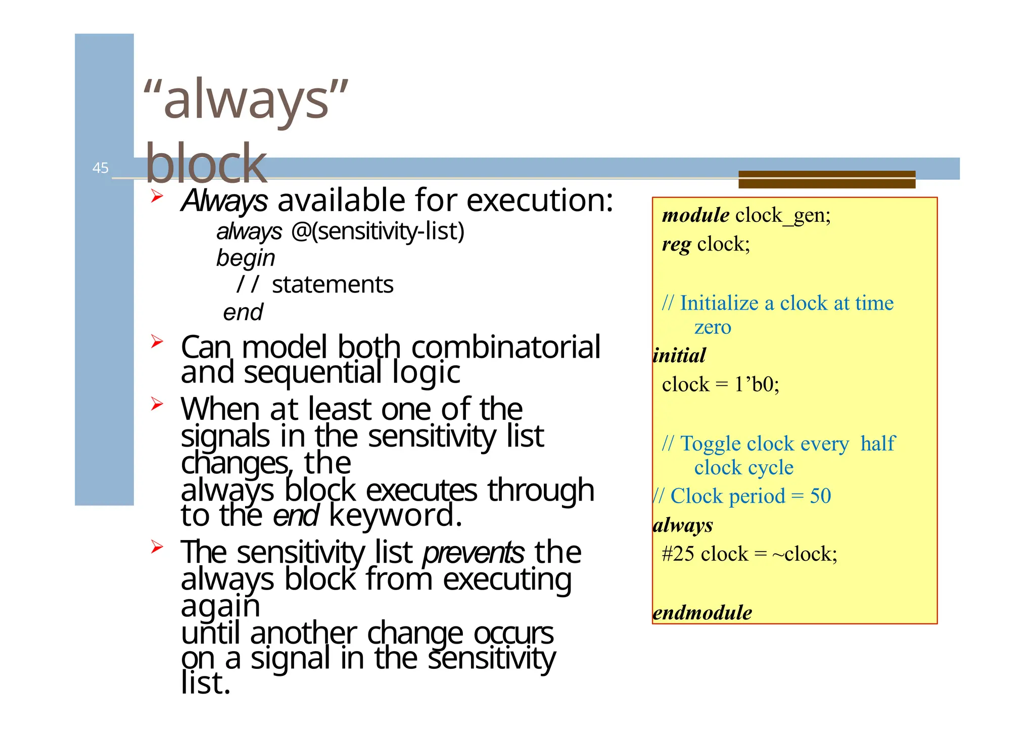
44. “always”
block
45
 Always available for execution:
always @(sensitivity-list)
begin
/ / statements
end
 Can model both combinatorial
and sequential logic
 When at least one of the
signals in the sensitivity list
changes, the
always block executes through
to the end keyword.
 The sensitivity list prevents the
always block from executing
again
until another change occurs
on a signal in the sensitivity
list.
module clock_gen;
reg clock;
// Initialize a clock at time
zero
initial
clock = 1’b0;
// Toggle clock every half
clock cycle
// Clock period = 50
always
#25 clock = ~clock;
endmodule

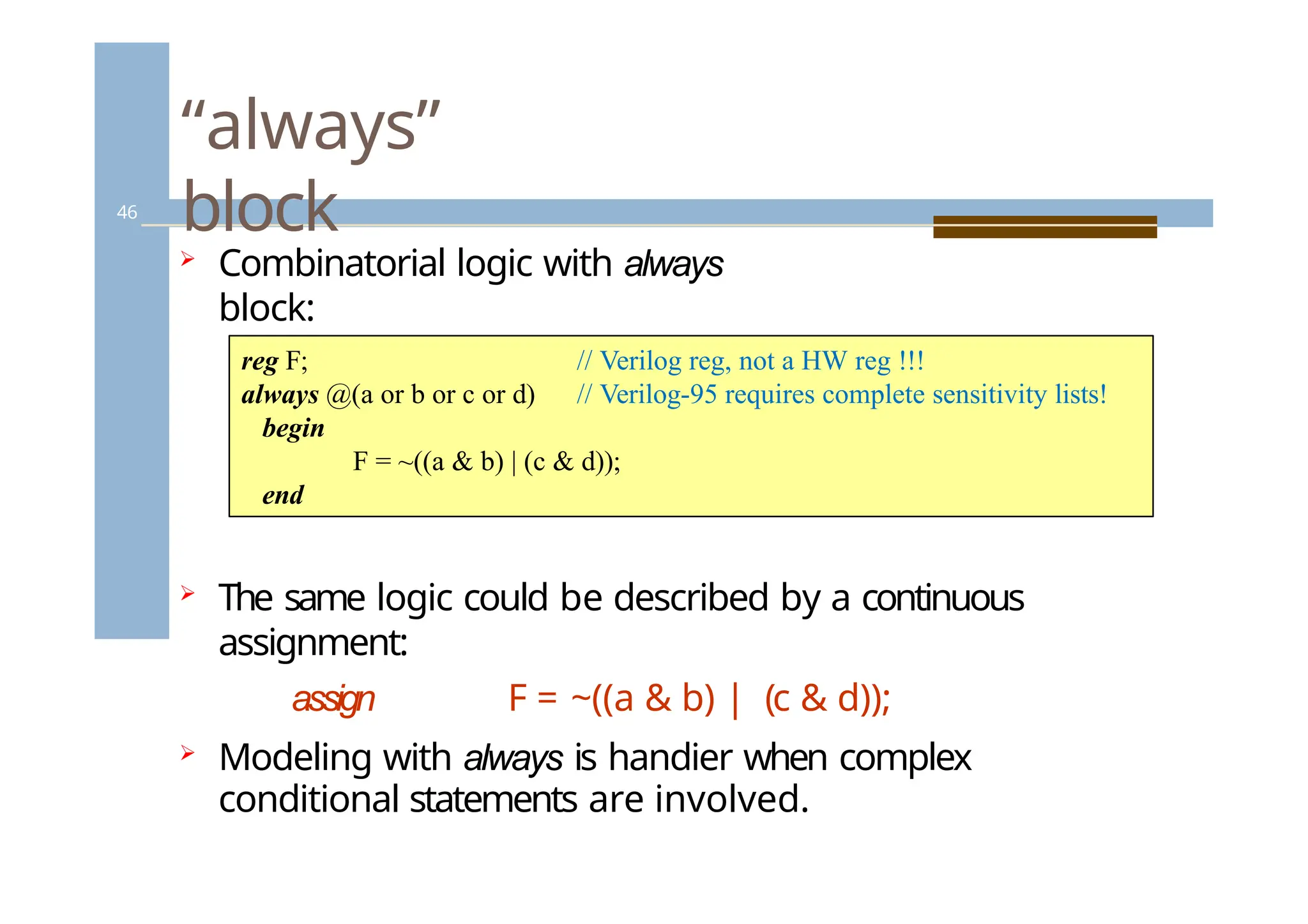
45. “always”
block
46
 Combinatorial logic with always
block:
// Verilog reg, not a HW reg !!!
// Verilog-95 requires complete sensitivity lists!
reg F;
always @(a or b or c or d)
begin
F = ~((a & b) | (c & d));
end
 The same logic could be described by a continuous
assignment:
assign F = ~((a & b) | (c & d));
 Modeling with always is handier when complex
conditional statements are involved.

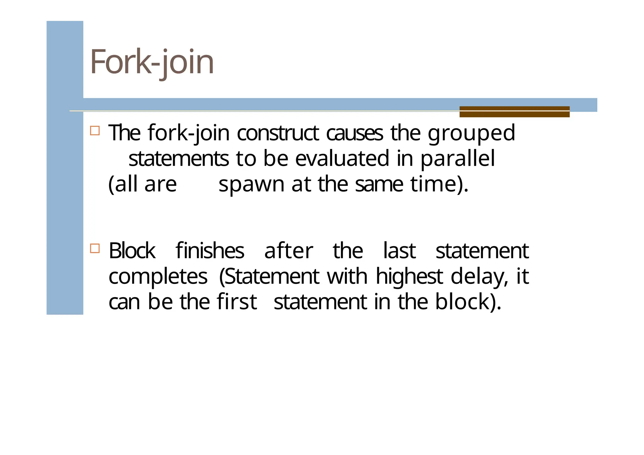
46. Fork-join
 The fork-join construct causes the grouped
statements to be evaluated in parallel
(all are spawn at the same time).
 Block finishes after the last statement
completes (Statement with highest delay, it
can be the first statement in the block).

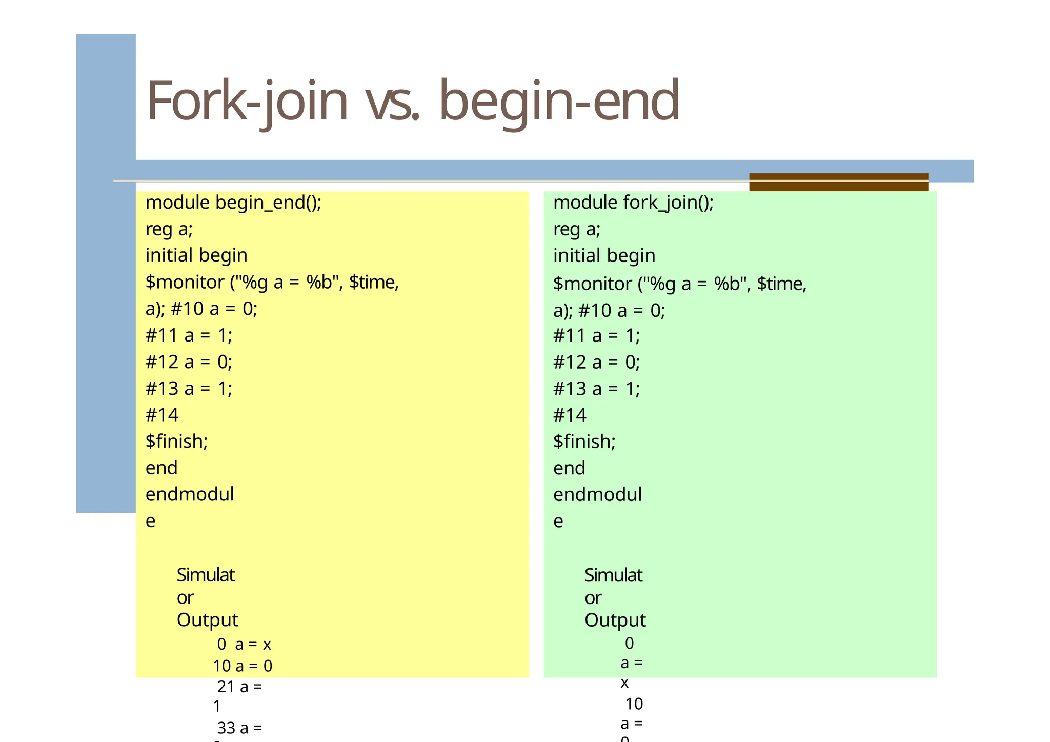
47. Fork-join vs. begin-end
module begin_end();
reg a;
initial begin
$monitor ("%g a = %b", $time,
a); #10 a = 0;
#11 a = 1;
#12 a = 0;
#13 a = 1;
#14
$finish;
end
endmodul
e
Simulat
or
Output
0 a = x
10 a = 0
21 a =
1
33 a =
module fork_join();
reg a;
initial begin
$monitor ("%g a = %b", $time,
a); #10 a = 0;
#11 a = 1;
#12 a = 0;
#13 a = 1;
#14
$finish;
end
endmodul
e
Simulat
or
Output
0
a =
x
10
a =

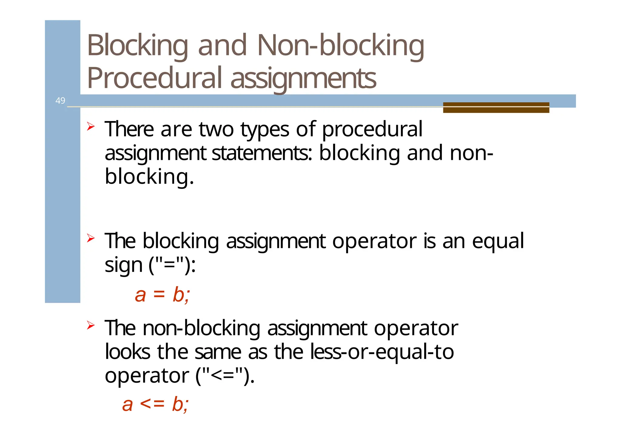
48. Blocking and Non-blocking
Procedural assignments
49
 There are two types of procedural
assignment statements: blocking and non-
blocking.
 The blocking assignment operator is an equal
sign ("="):
a = b;
 The non-blocking assignment operator
looks the same as the less-or-equal-to
operator ("<=").
a <= b;

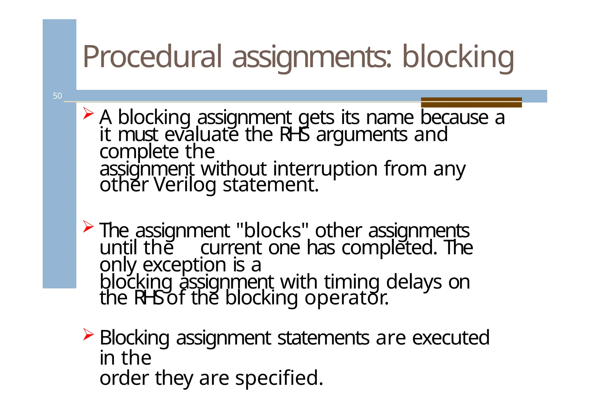
49. Procedural assignments: blocking
50
 A blocking assignment gets its name because a
it must evaluate the RHS arguments and
complete the
assignment without interruption from any
other Verilog statement.
 The assignment "blocks" other assignments
until the current one has completed. The
only exception is a
blocking assignment with timing delays on
the RHSof the blocking operator.
 Blocking assignment statements are executed
in the
order they are specified.

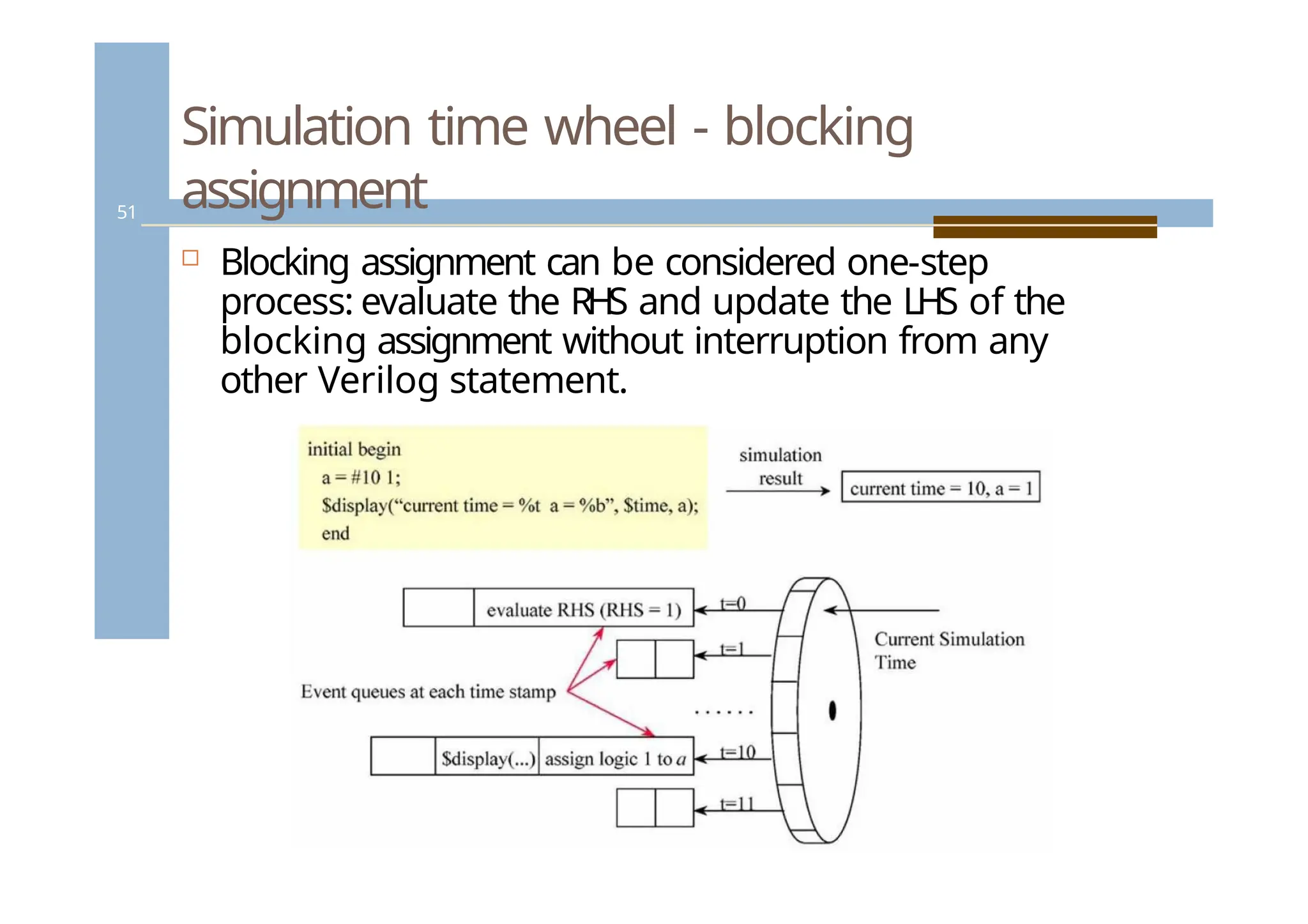
50. Simulation time wheel - blocking
assignment
 Blocking assignment can be considered one-step
process: evaluate the RHS and update the LHS of the
blocking assignment without interruption from any
other Verilog statement.
51

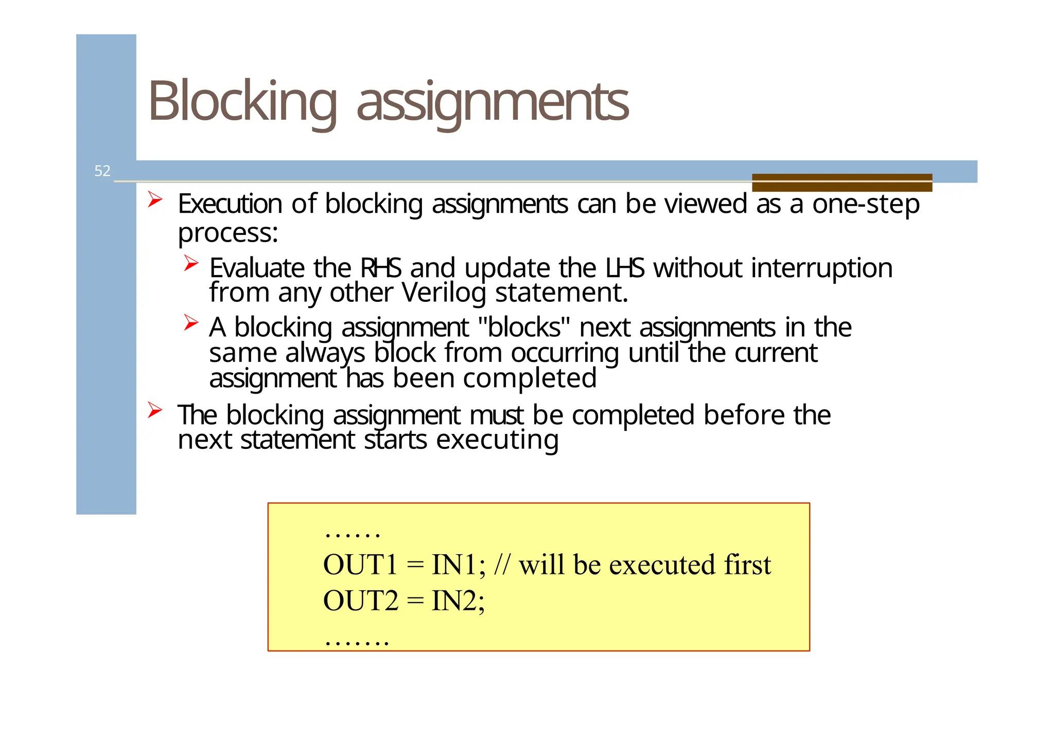
51. Blocking assignments
52
 Execution of blocking assignments can be viewed as a one-step
process:
 Evaluate the RHS and update the LHS without interruption
from any other Verilog statement.
 A blocking assignment "blocks" next assignments in the
same always block from occurring until the current
assignment has been completed
 The blocking assignment must be completed before the
next statement starts executing
……
OUT1 = IN1; // will be executed first
OUT2 = IN2;
…….

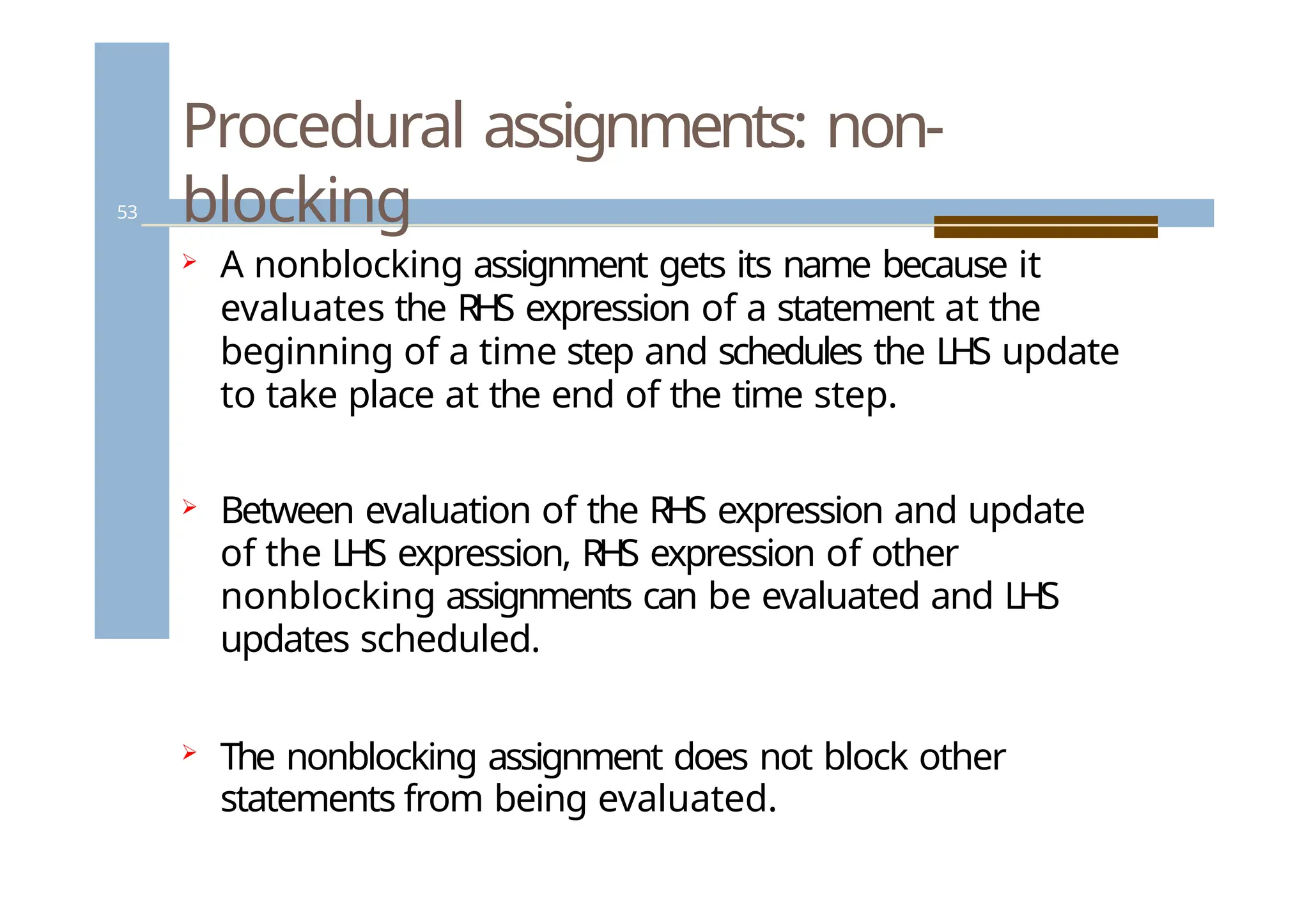
52. Procedural assignments: non-
blocking
53
 A nonblocking assignment gets its name because it
evaluates the RHS expression of a statement at the
beginning of a time step and schedules the LHS update
to take place at the end of the time step.
 Between evaluation of the RHS expression and update
of the LHS expression, RHS expression of other
nonblocking assignments can be evaluated and LHS
updates scheduled.
 The nonblocking assignment does not block other
statements from being evaluated.

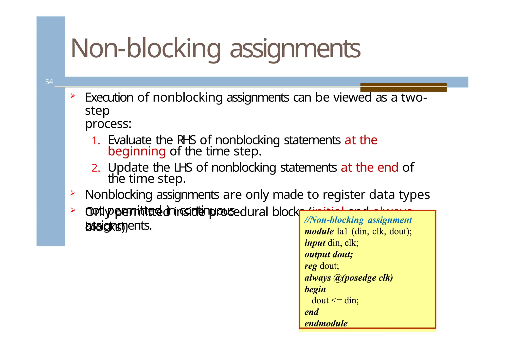
53. Non-blocking assignments
54
 Execution of nonblocking assignments can be viewed as a two-
step
process:
1. Evaluate the RHS of nonblocking statements at the
beginning of the time step.
2. Update the LHS of nonblocking statements at the end of
the time step.
 Nonblocking assignments are only made to register data types
 Only permitted inside procedural blocks (initial and always
blocks),
not permitted in continuous
assignments.
//Non-blocking assignment
module la1 (din, clk, dout);
input din, clk;
output dout;
reg dout;
always @(posedge clk)
begin
dout <= din;
end
endmodule

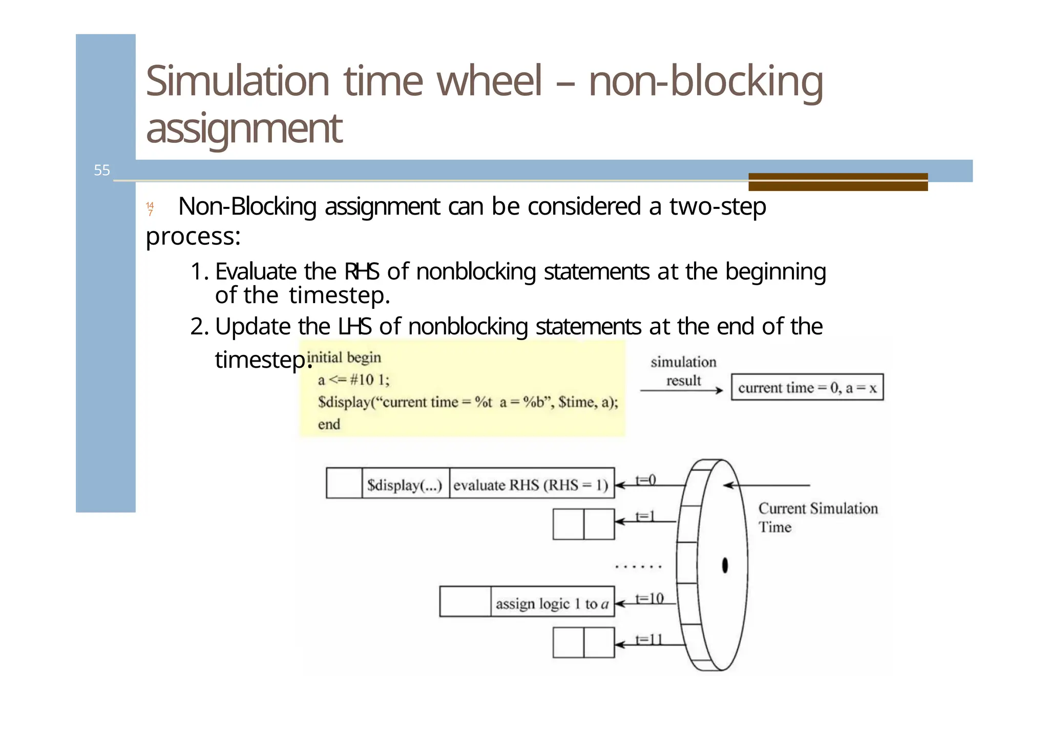
54. Simulation time wheel – non-blocking
assignment
 Non-Blocking assignment can be considered a two-step
process:
1. Evaluate the RHS of nonblocking statements at the beginning
of the timestep.
2. Update the LHS of nonblocking statements at the end of the
timestep.
55

55. Procedural blocks
56
 Procedural blocks have the following
components:
 Procedural assignment statements
 High-level constructs (loops, conditional
statements)
 Timing controls

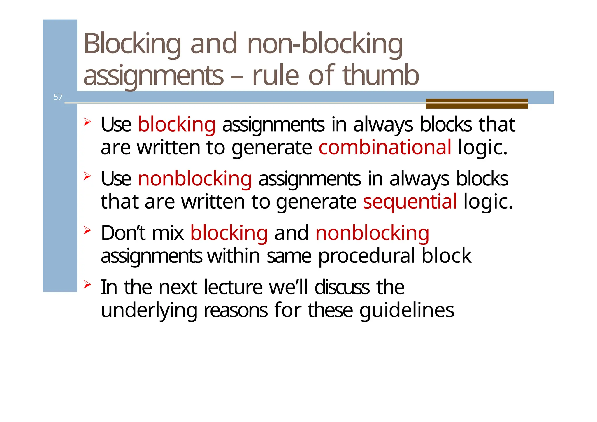
56. Blocking and non-blocking
assignments – rule of thumb
57
 Use blocking assignments in always blocks that
are written to generate combinational logic.
 Use nonblocking assignments in always blocks
that are written to generate sequential logic.
 Don’t mix blocking and nonblocking
assignments within same procedural block
 In the next lecture we’ll discuss the
underlying reasons for these guidelines

57. Blocking and non-blocking
assignments
58
// Bad code - potential simulation race
module pipeb1 (q3, d, clk);
output [7:0] q3;
input [7:0] d;
input clk;
reg [7:0] q3, q2, q1;
always @(posedge clk) begin
q1 = d;
q2 = q1;
q3 = q2;
end
endmodule
// Good code
module pipen1 (q3, d, clk);
output [7:0] q3;
input [7:0] d;
input clk;
reg [7:0] q3, q2, q1;
always @(posedge clk) begin
q1 <= d;
q2 <= q1;
q3 <= q2;
end
endmodule

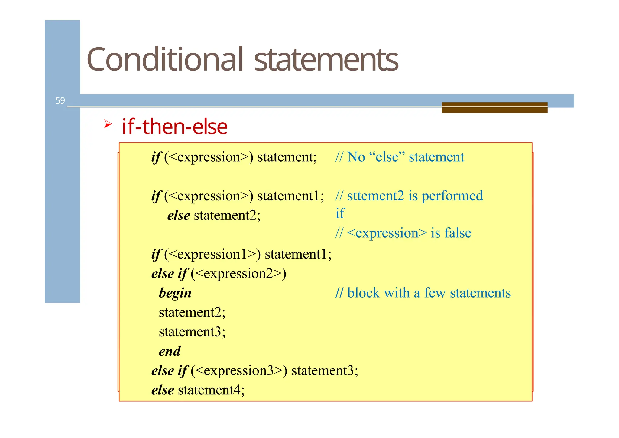
58. Conditional statements
59
 if-then-else
construct:
if (<expression>) statement; // No “else” statement
if (<expression>) statement1;
else statement2;
// sttement2 is performed
if
// <expression> is false
// block with a few statements
if (<expression1>) statement1;
else if (<expression2>)
begin
statement2;
statement3;
end
else if (<expression3>) statement3;
else statement4;

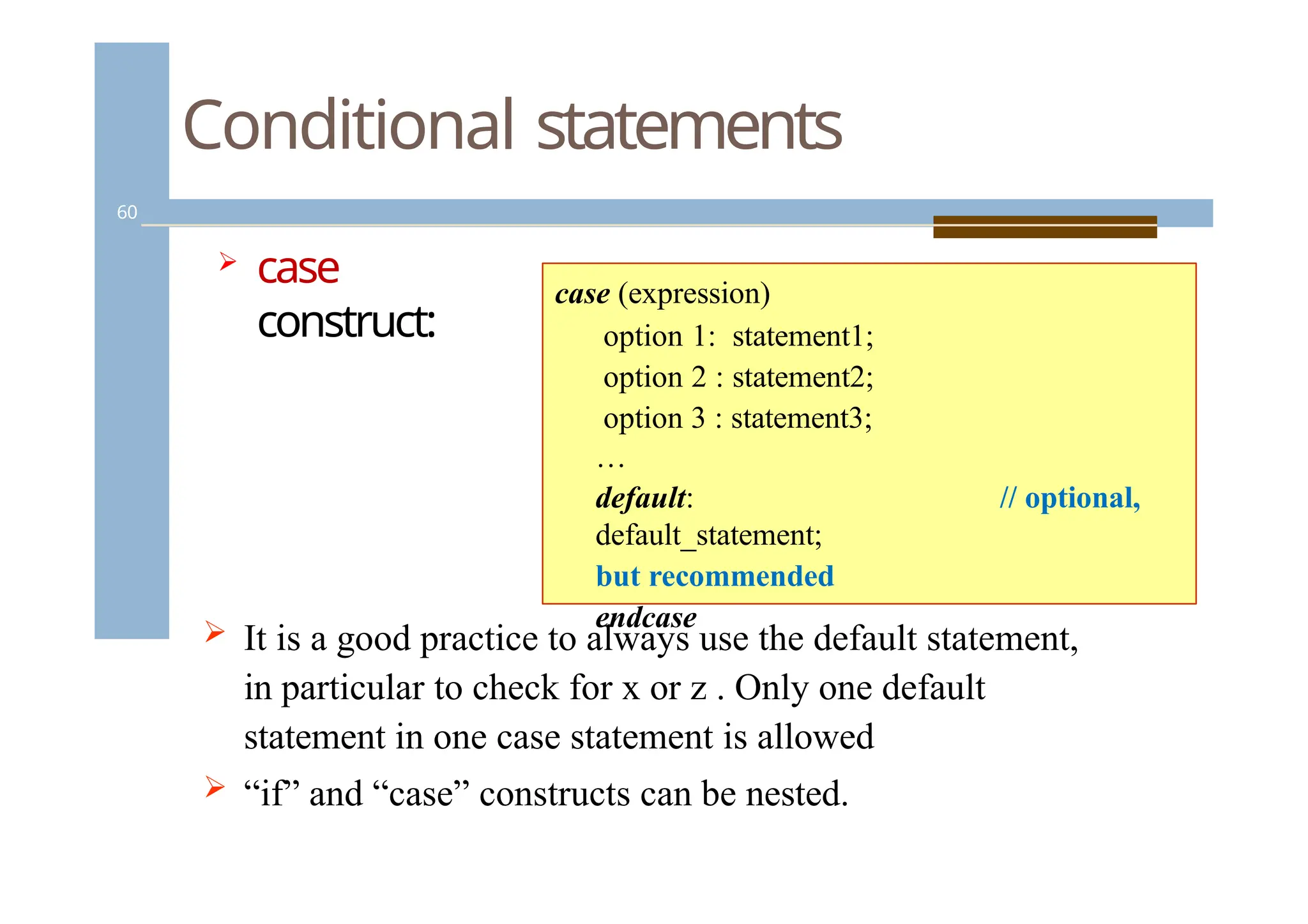
59. Conditional statements
60
 case
construct:
// optional,
case (expression)
option 1: statement1;
option 2 : statement2;
option 3 : statement3;
…
default:
default_statement;
but recommended
endcase
 It is a good practice to always use the default statement,
in particular to check for x or z . Only one default
statement in one case statement is allowed
 “if” and “case” constructs can be nested.

60. i1
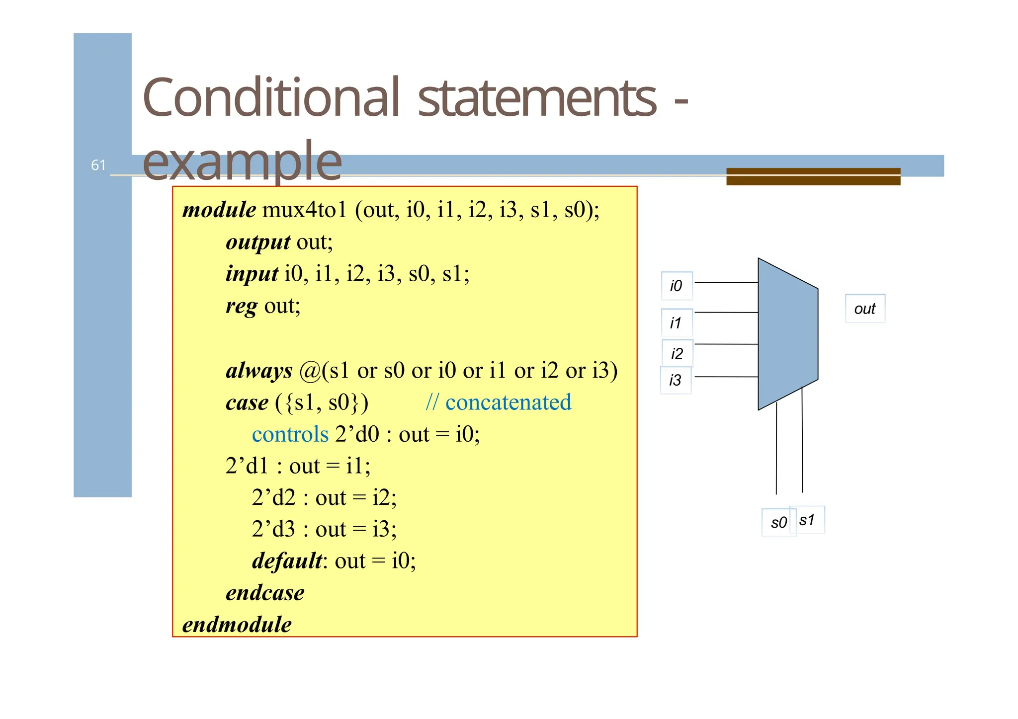
Conditional statements -
example
61
module mux4to1 (out, i0, i1, i2, i3, s1, s0);
output out;
input i0, i1, i2, i3, s0, s1;
reg out;
always @(s1 or s0 or i0 or i1 or i2 or i3)
case ({s1, s0}) // concatenated
controls 2’d0 : out = i0;
2’d1 : out = i1;
2’d2 : out = i2;
2’d3 : out = i3;
default: out = i0;
endcase
endmodule
i0
i2
i3
out
s0 s1

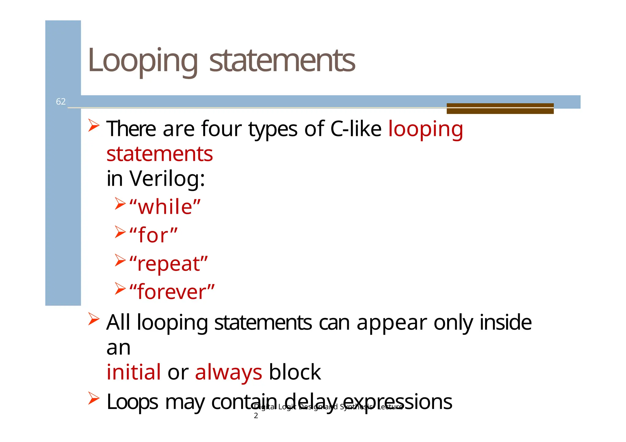
61. Looping statements
62
 There are four types of C-like looping
statements
in Verilog:
“while”
“for”
“repeat”
“forever”
 All looping statements can appear only inside
an
initial or always block
 Loops may contain delay expressions
Digital Logic Design and Synthesis- Lecture
2

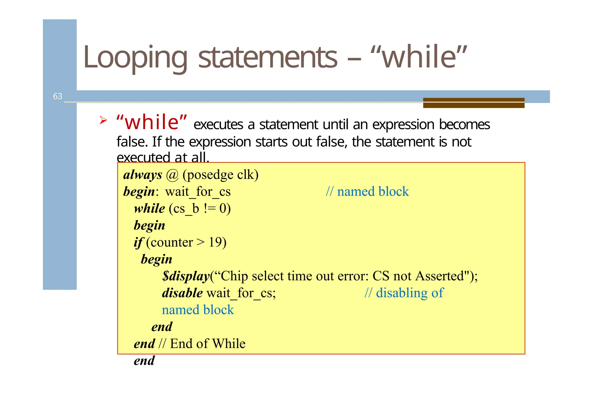
62. Looping statements – “while”
63
 “while” executes a statement until an expression becomes
false. If the expression starts out false, the statement is not
executed at all.
// named block
always @ (posedge clk)
begin: wait_for_cs
while (cs_b != 0)
begin
if (counter > 19)
begin
$display(“Chip select time out error: CS not Asserted");
disable wait_for_cs; // disabling of
named block
end
end // End of While
end

63. Looping statements – “for”
64
 The “for” statement initializes a variable, evaluates the
expression (exits the loop, if false), and executes as
assignment, all in a single statement.
 For loops are generally used when there is a fixed
beginning and end to the loop. If the loop is simply
looping on a certain condition, it is preferable to use
while
begin :count1s
reg [7:0] tmp;
for (tmp = rega; tmp; tmp = tmp >>
1)
if (tmp]) count = count + 1;
end
tmp = 8’b11111111; count = 0;
initial
condition check
control variable
assignment

64. Looping statements – “repeat”
65
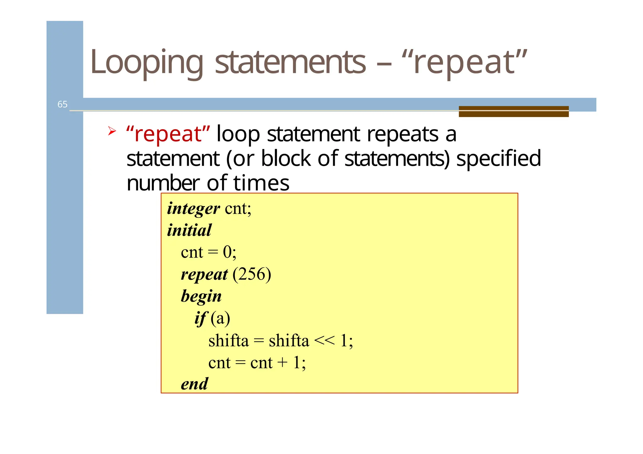
 “repeat” loop statement repeats a
statement (or block of statements) specified
number of times
integer cnt;
initial
cnt = 0;
repeat (256)
begin
if (a)
shifta = shifta << 1;
cnt = cnt + 1;
end

65. Looping statements – “forever”
66
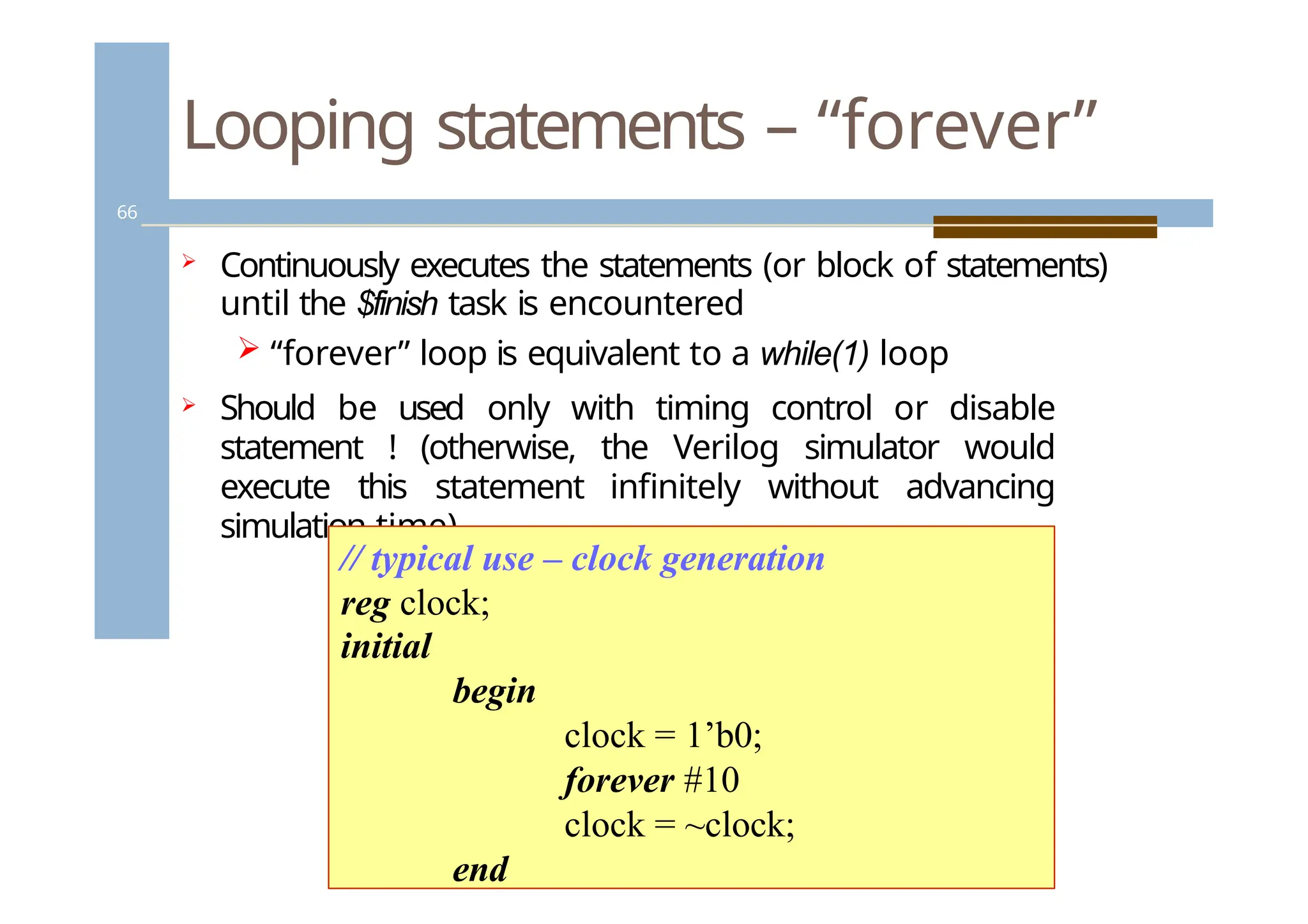
 Continuously executes the statements (or block of statements)
until the $finish task is encountered
 “forever” loop is equivalent to a while(1) loop
 Should be used only with timing control or disable
statement ! (otherwise, the Verilog simulator would
execute this statement infinitely without advancing
simulation time)
// typical use – clock generation
reg clock;
initial
begin
clock = 1’b0;
forever #10
clock = ~clock;
end

66. Timing
control
67
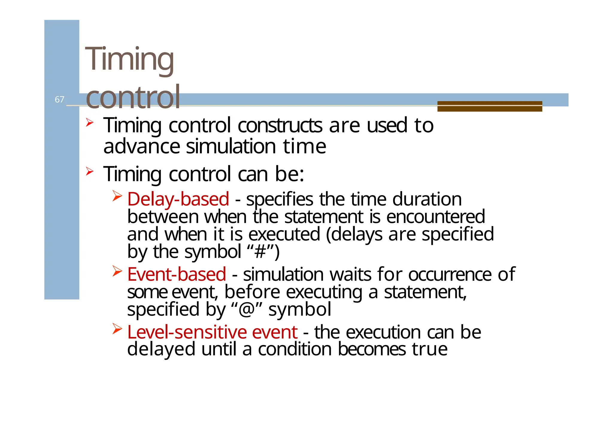
 Timing control constructs are used to
advance simulation time
 Timing control can be:
 Delay-based - specifies the time duration
between when the statement is encountered
and when it is executed (delays are specified
by the symbol “#”)
 Event-based - simulation waits for occurrence of
someevent, before executing a statement,
specified by “@” symbol
 Level-sensitive event - the execution can be
delayed until a condition becomes true

67. Delay based timing control
68
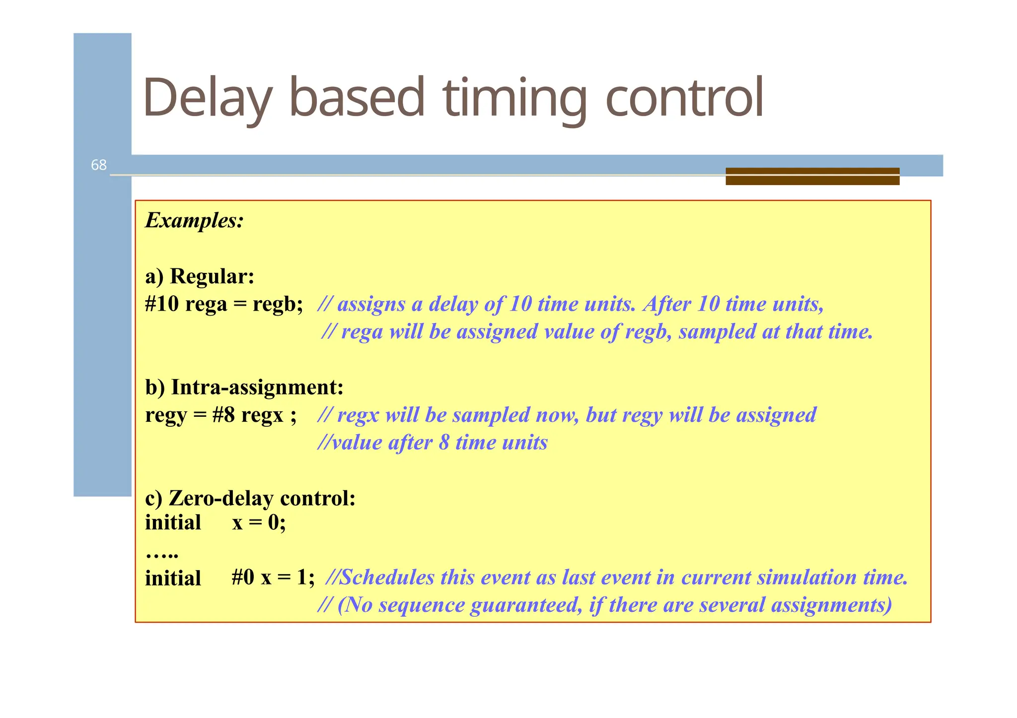
Examples:
a) Regular:
#10 rega = regb; // assigns a delay of 10 time units. After 10 time units,
// rega will be assigned value of regb, sampled at that time.
b) Intra-assignment:
regy = #8 regx ; // regx will be sampled now, but regy will be assigned
//value after 8 time units
c) Zero-delay control:
x = 0;
initial
…..
initial #0 x = 1; //Schedules this event as last event in current simulation time.
// (No sequence guaranteed, if there are several assignments)

68. Event based timing
control
69
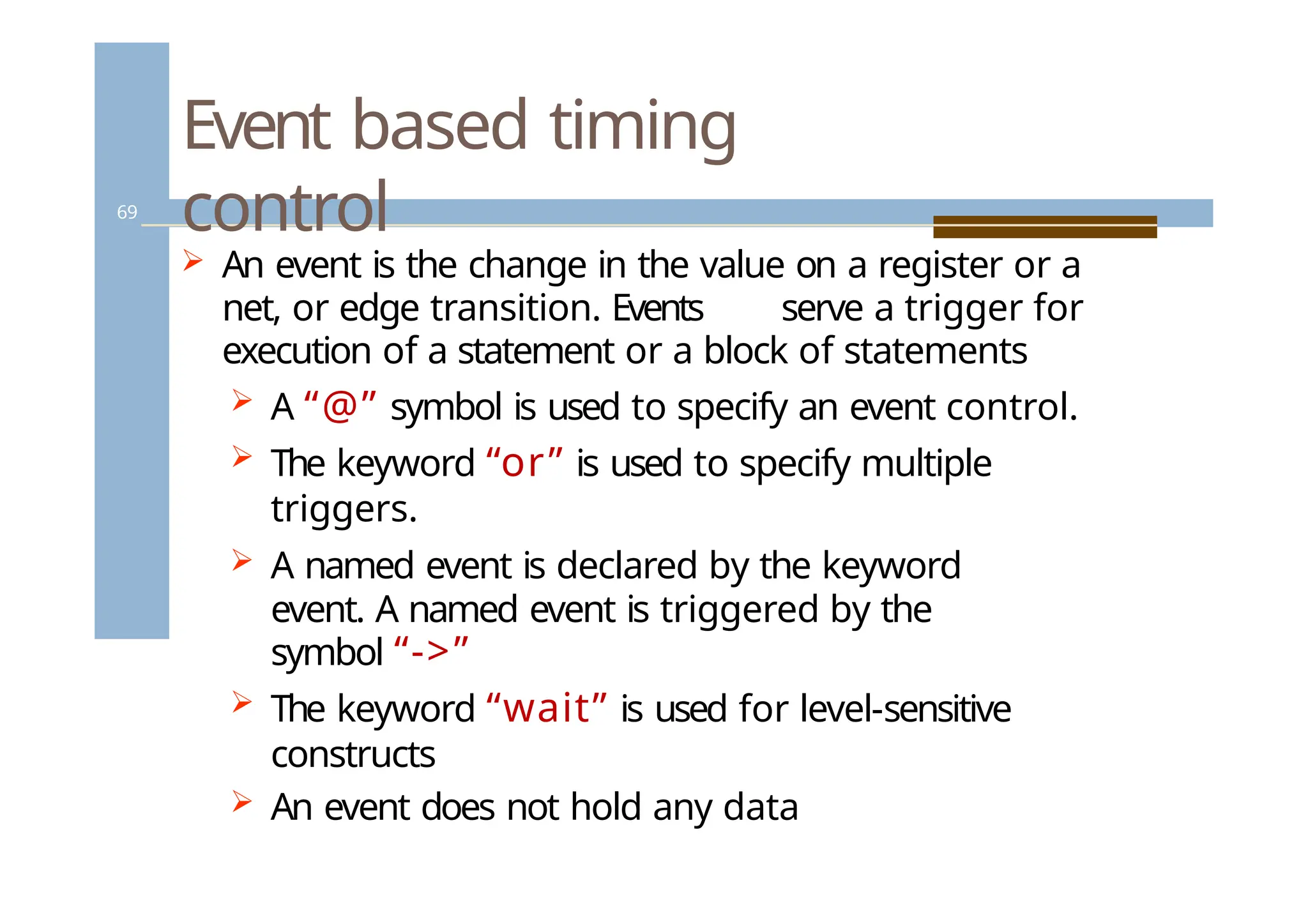
 An event is the change in the value on a register or a
net, or edge transition. Events serve a trigger for
execution of a statement or a block of statements
 A “@” symbol is used to specify an event control.
 The keyword “or” is used to specify multiple
triggers.
 A named event is declared by the keyword
event. A named event is triggered by the
symbol “->”
 The keyword “wait” is used for level-sensitive
constructs
 An event does not hold any data

69. Event based timing
control
70
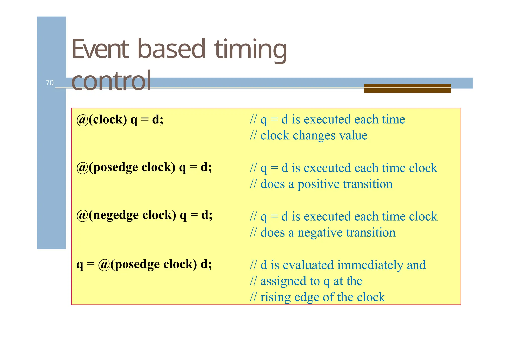
@(clock) q = d;
@(posedge clock) q = d;
@(negedge clock) q = d;
q = @(posedge clock) d;
// q = d is executed each time
// clock changes value
// q = d is executed each time clock
// does a positive transition
// q = d is executed each time clock
// does a negative transition
// d is evaluated immediately and
// assigned to q at the
// rising edge of the clock

70. Event based timing
control
71
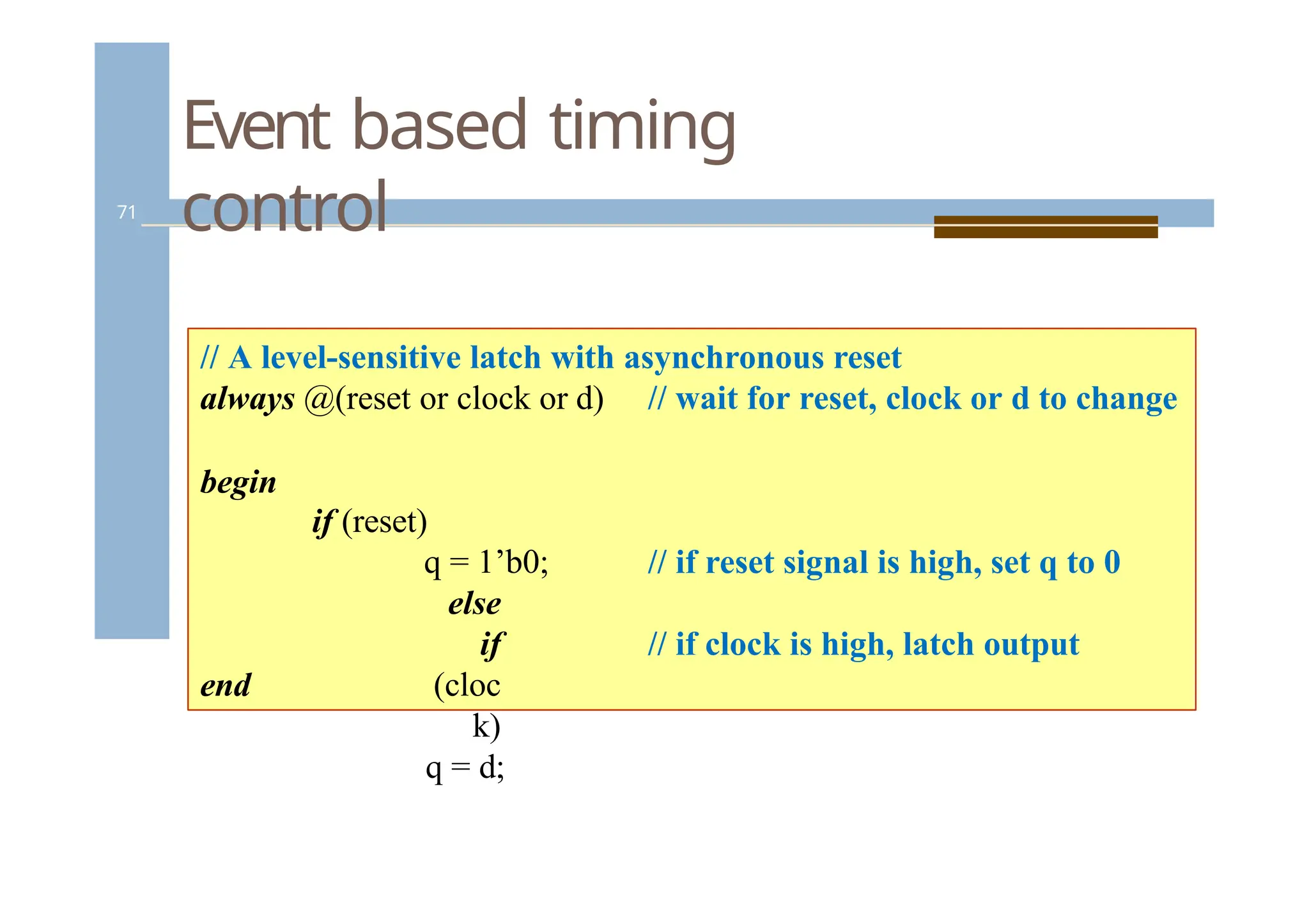
// A level-sensitive latch with asynchronous reset
always @(reset or clock or d) // wait for reset, clock or d to change
begin
// if reset signal is high, set q to 0
if (reset)
q = 1’b0;
else
if
(cloc
k)
q = d;
// if clock is high, latch output
end

71. Event based timing
control
72
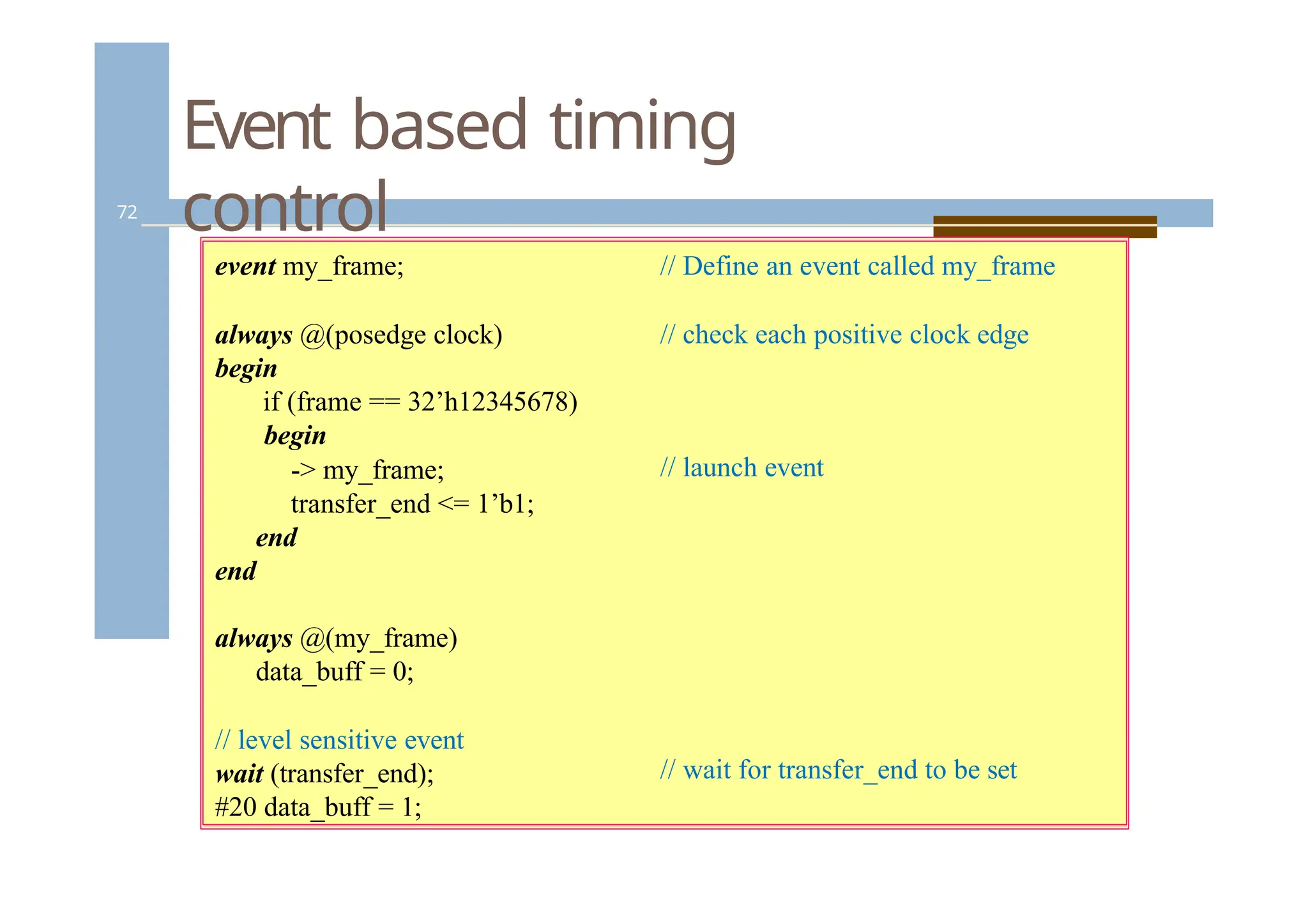
// Define an event called my_frame
// check each positive clock edge
// launch event
// wait for transfer_end to be set
event my_frame;
always @(posedge clock)
begin
if (frame == 32’h12345678)
begin
-> my_frame;
transfer_end <= 1’b1;
end
end
always @(my_frame)
data_buff = 0;
// level sensitive event
wait (transfer_end);
#20 data_buff = 1;

72. Compiler directives
73
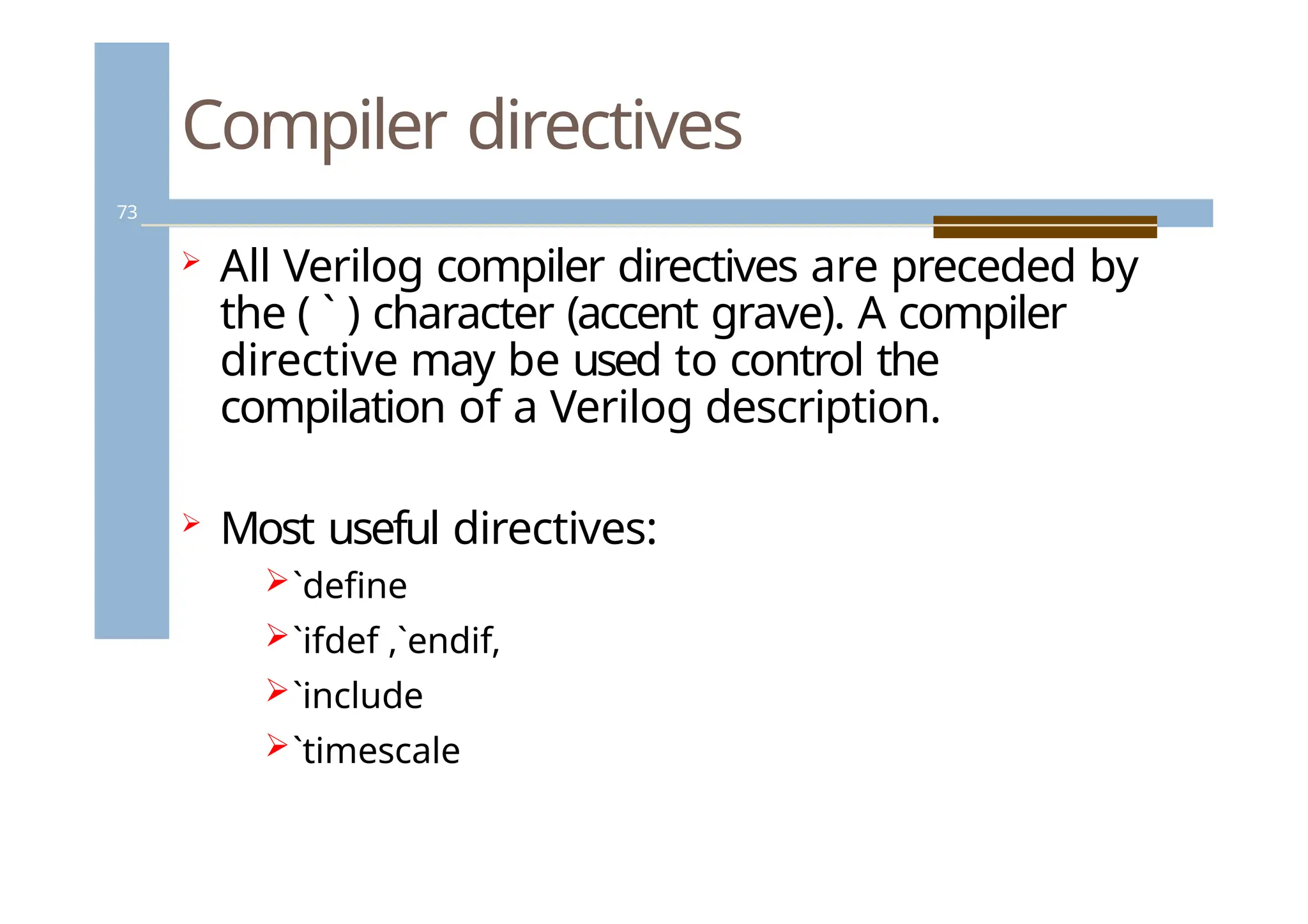
 All Verilog compiler directives are preceded by
the ( ` ) character (accent grave). A compiler
directive may be used to control the
compilation of a Verilog description.
 Most useful directives:
`define
`ifdef ,`endif,
`include
`timescale

73. Compiler directives – text
substitution
74
`define WORD_SIZE 64
`define byte_reg reg[7:0]
`define one 1’b1
`define F $finish
// Text substitution
// Define a frequently used text
// Improve readability
// Create a command alias

74. Compiler directives – text substitution
75
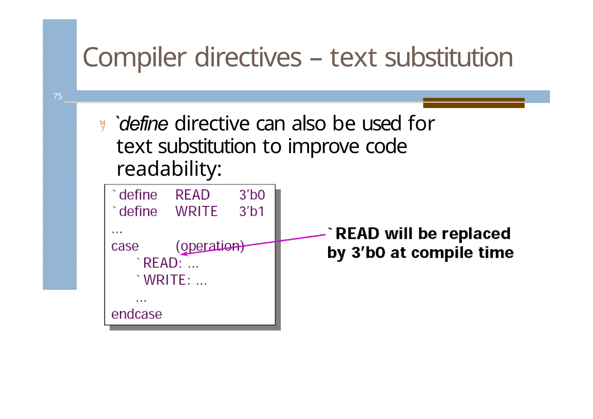
 `define directive can also be used for
text substitution to improve code
readability:

75. Compiler directives – conditional
compilation
76
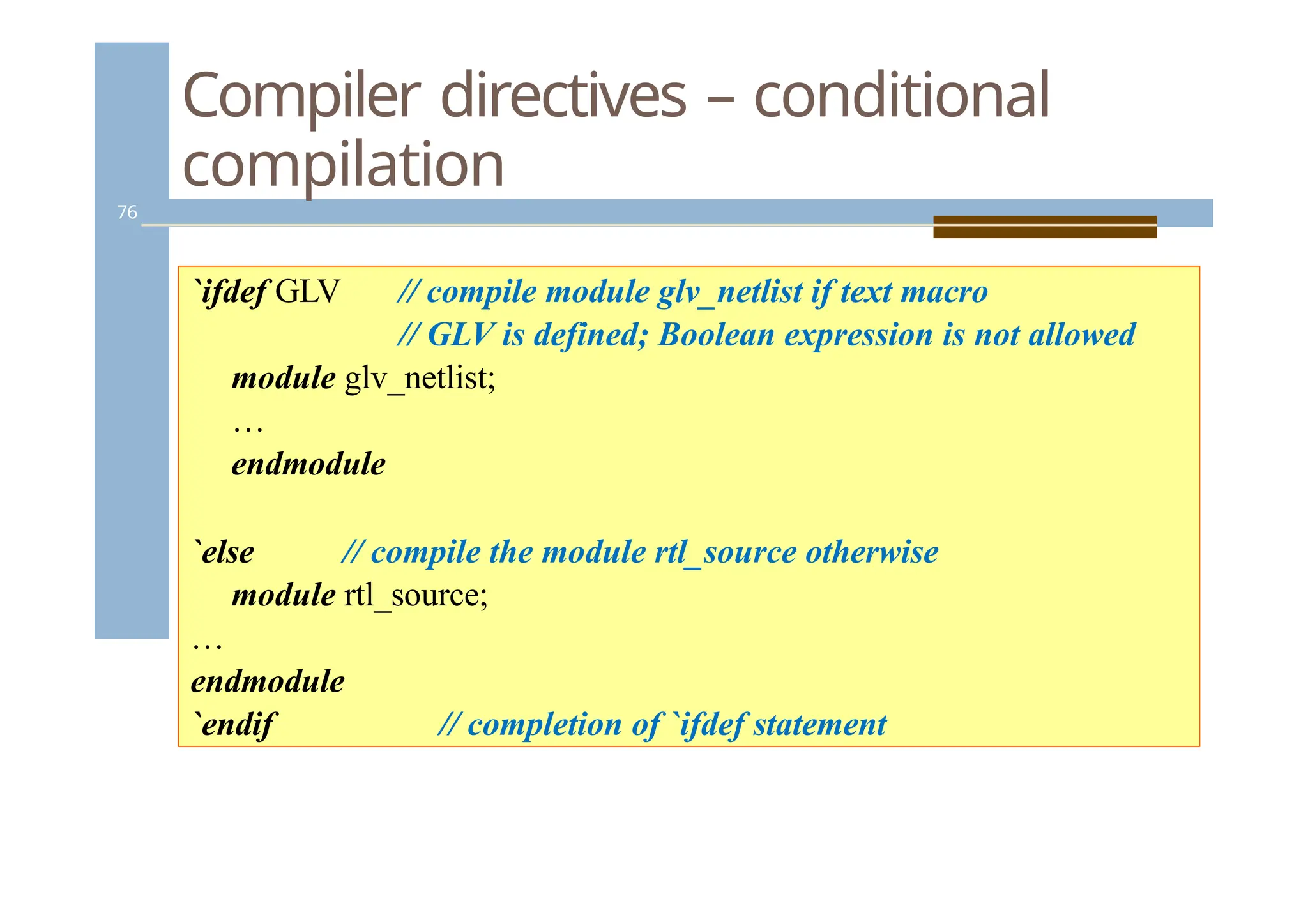
`ifdef GLV // compile module glv_netlist if text macro
// GLV is defined; Boolean expression is not allowed
module glv_netlist;
…
endmodule
`else // compile the module rtl_source otherwise
module rtl_source;
…
endmodule
`endif // completion of `ifdef statement

76. Compiler directives – code
inclusion
77
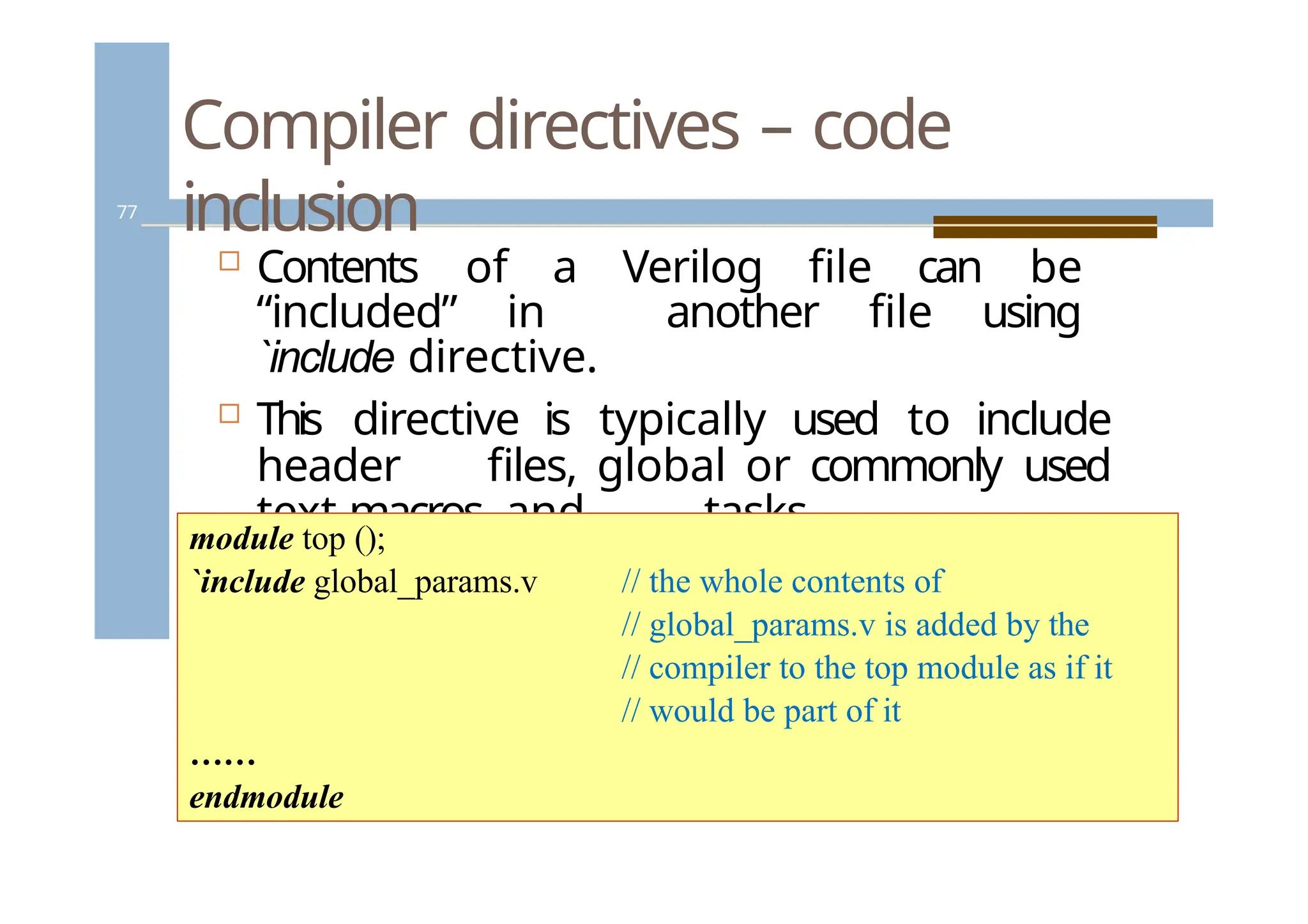
 Contents of a Verilog file can be
“included” in another file using
`include directive.
 This directive is typically used to include
header files, global or commonly used
text macros, and tasks.
module top ();
`include global_params.v // the whole contents of
// global_params.v is added by the
// compiler to the top module as if it
// would be part of it
……
endmodule

77. Compiler directives - timescale
78
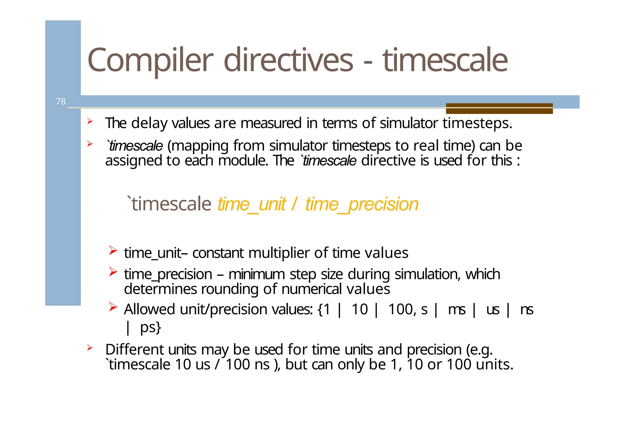
 The delay values are measured in terms of simulator timesteps.
 `timescale (mapping from simulator timesteps to real time) can be
assigned to each module. The `timescale directive is used for this :
`timescale time_unit / time_precision
 time_unit– constant multiplier of time values
 time_precision – minimum step size during simulation, which
determines rounding of numerical values
 Allowed unit/precision values: {1 | 10 | 100, s | ms | us | ns
| ps}
 Different units may be used for time units and precision (e.g.
`timescale 10 us / 100 ns ), but can only be 1, 10 or 100 units.

78. Compiler directives - timescale
79
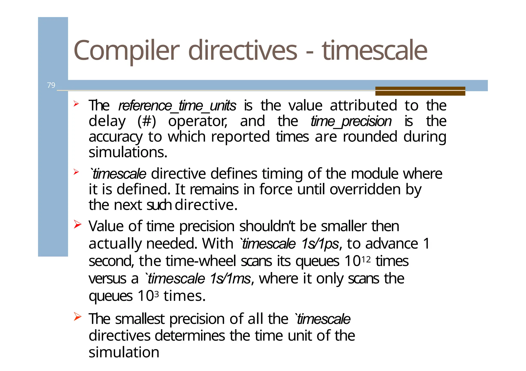
 The reference_time_units is the value attributed to the
delay (#) operator, and the time_precision is the
accuracy to which reported times are rounded during
simulations.
 `timescale directive defines timing of the module where
it is defined. It remains in force until overridden by
the next suchdirective.
 Value of time precision shouldn’t be smaller then
actually needed. With `timescale 1s/1ps, to advance 1
second, the time-wheel scans its queues 1012 times
versus a `timescale 1s/1ms, where it only scans the
queues 103 times.
 The smallest precision of all the `timescale
directives determines the time unit of the
simulation

79. Compiler directives - timescale
80
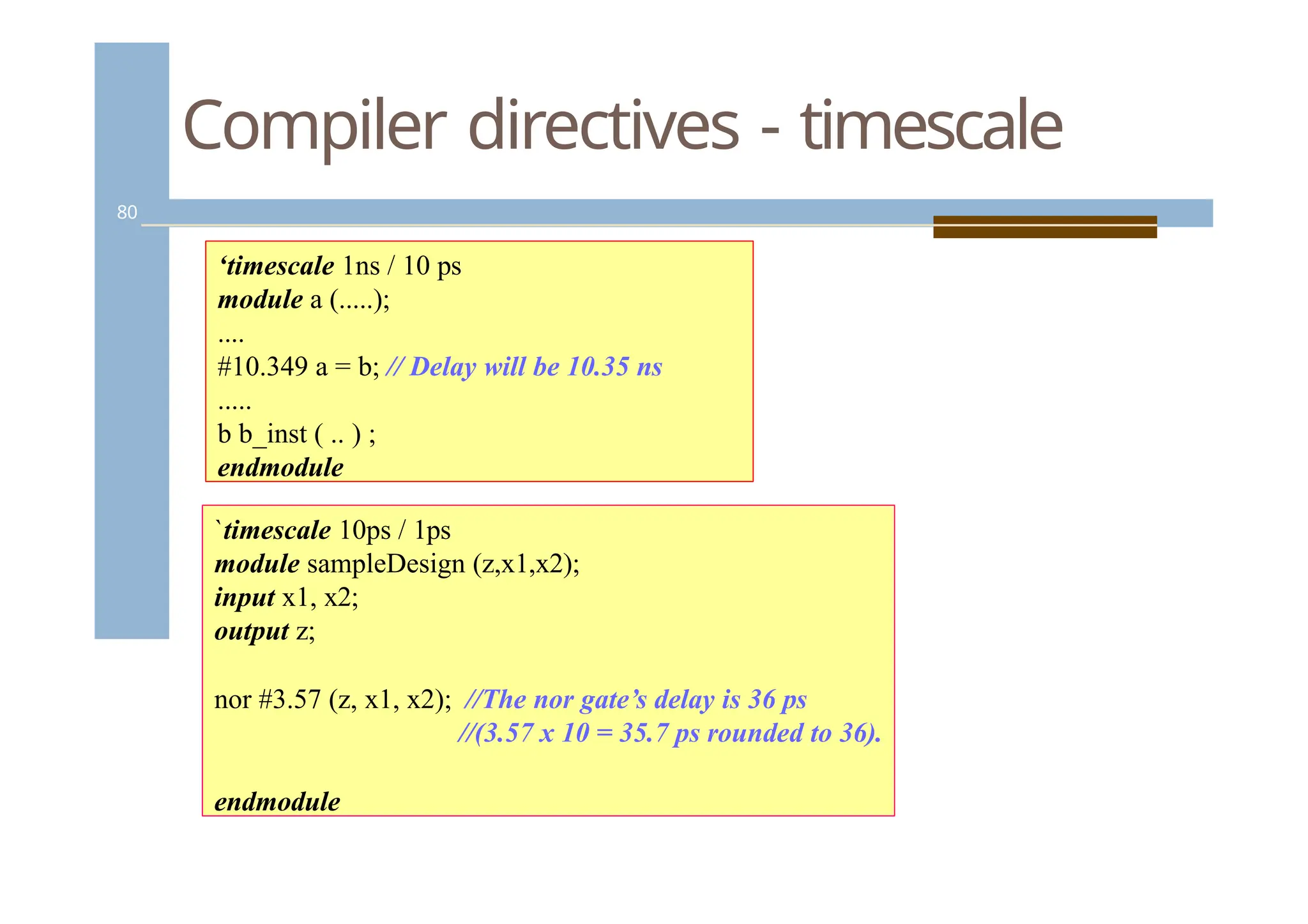
‘timescale 1ns / 10 ps
module a (.....);
....
#10.349 a = b; // Delay will be 10.35 ns
.....
b b_inst ( .. ) ;
endmodule
`timescale 10ps / 1ps
module sampleDesign (z,x1,x2);
input x1, x2;
output z;
nor #3.57 (z, x1, x2); //The nor gate’s delay is 36 ps
//(3.57 x 10 = 35.7 ps rounded to 36).
endmodule

80. Tasks and functions
81
 Often it is required to implement the
same functionality at many places in a
design.
 Rather than replicating the code, a routine
should be invoked each time when the
same functionality is called.
 T
asks and functions allow the designer to
abstract Verilog code that is used at many
places in the design.
 T
asks and functions are included in the design
hierarchy. Like named blocks, tasks and
functions can be addressed by means of
hierarchical names

81. Tasks and functions
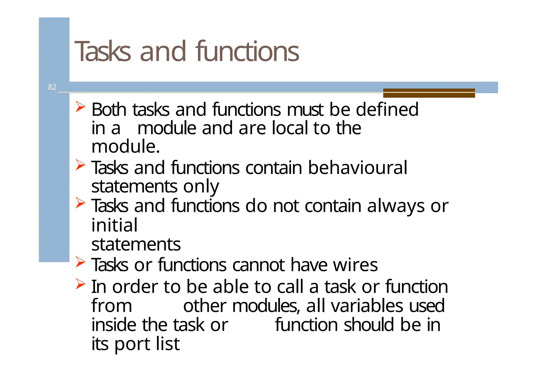
82
 Both tasks and functions must be defined
in a module and are local to the
module.
 T
asks and functions contain behavioural
statements only
 T
asks and functions do not contain always or
initial
statements
 T
asks or functions cannot have wires
 In order to be able to call a task or function
from other modules, all variables used
inside the task or function should be in
its port list

82. Tasks and functions
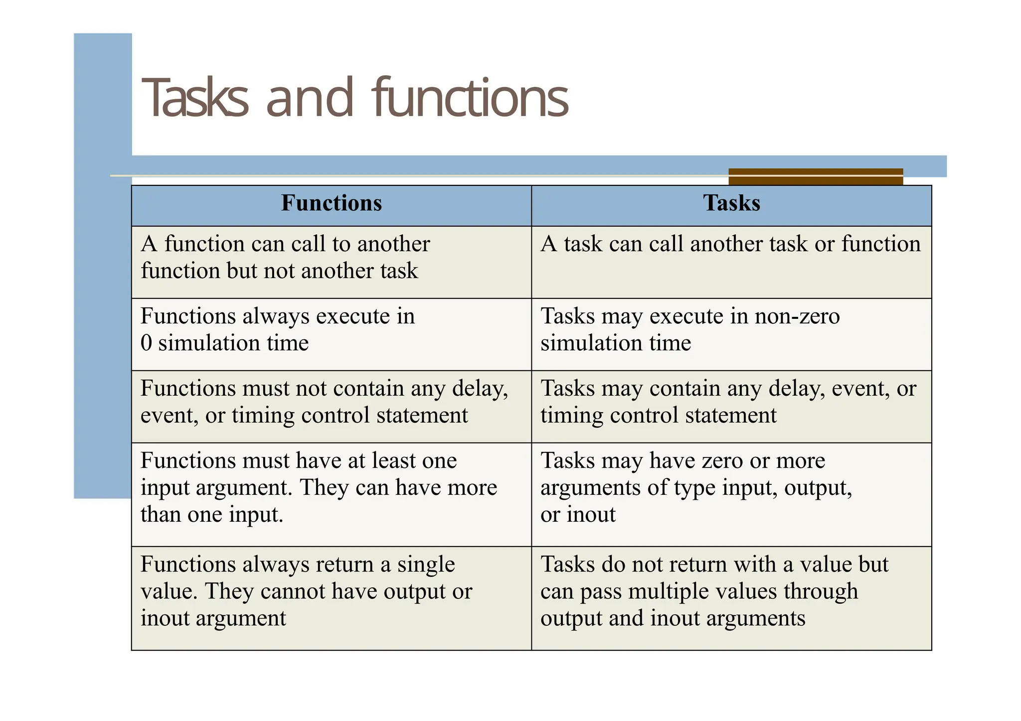
Functions Tasks
A function can call to another
function but not another task
A task can call another task or function
Functions always execute in
0 simulation time
Tasks may execute in non-zero
simulation time
Functions must not contain any delay,
event, or timing control statement
Tasks may contain any delay, event, or
timing control statement
Functions must have at least one
input argument. They can have more
than one input.
Tasks may have zero or more
arguments of type input, output,
or inout
Functions always return a single
value. They cannot have output or
inout argument
Tasks do not return with a value but
can pass multiple values through
output and inout arguments

83. Tasks and functions
84
// Example for function
function [31:0] factorial;
input [3:0] operand;
reg [3:0] index;
begin
factorial = operand ? 1 : 0;
for (index = 2; index <= operand; index = index +
1) factorial = index * factorial;
end
endfunction
// Calling
a function
for (n = 2;
n <= 9; n =
n+1)
begin
$display ("Partial result n=%d result=%d", n,
result); result = n * factorial(n) / ((n * 2) + 1);
end

84. Tasks and functions
85
//Example of Task Definition:
task light;
output color;
input [31:0] tics;
begin
repeat (tics)
@(posedge
clock);
color = off;
// turn light off
end
endtask
//
Invokin
g the
task in
the
module

85. System tasks
86
 All Verilog simulators support system tasks
used for some routine operations, like print,
stop/interrupt simulation, monitor variables,
dumping signal values etc.
 System tasks look like $<command>

86. System tasks
87
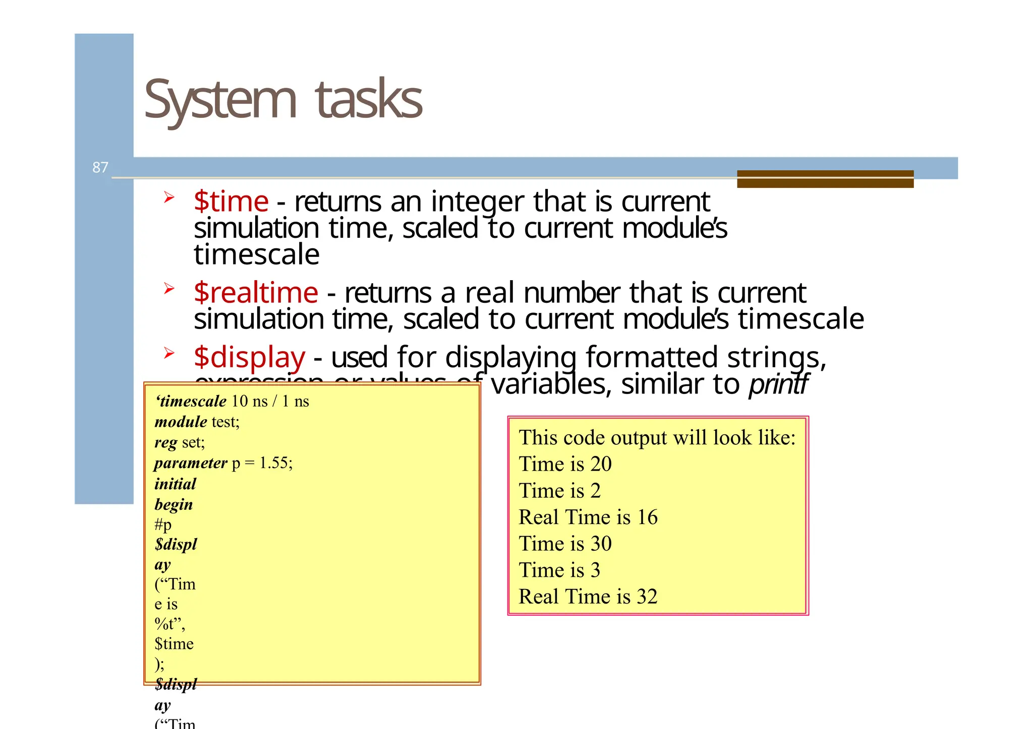
 $time - returns an integer that is current
simulation time, scaled to current module’s
timescale
 $realtime - returns a real number that is current
simulation time, scaled to current module’s timescale
 $display - used for displaying formatted strings,
expression or values of variables, similar to printf
in C.
‘timescale 10 ns / 1 ns
module test;
reg set;
parameter p = 1.55;
initial
begin
#p
$displ
ay
(“Tim
e is
%t”,
$time
);
$displ
ay
This code output will look like:
Time is 20
Time is 2
Real Time is 16
Time is 30
Time is 3
Real Time is 32

87. System tasks
88
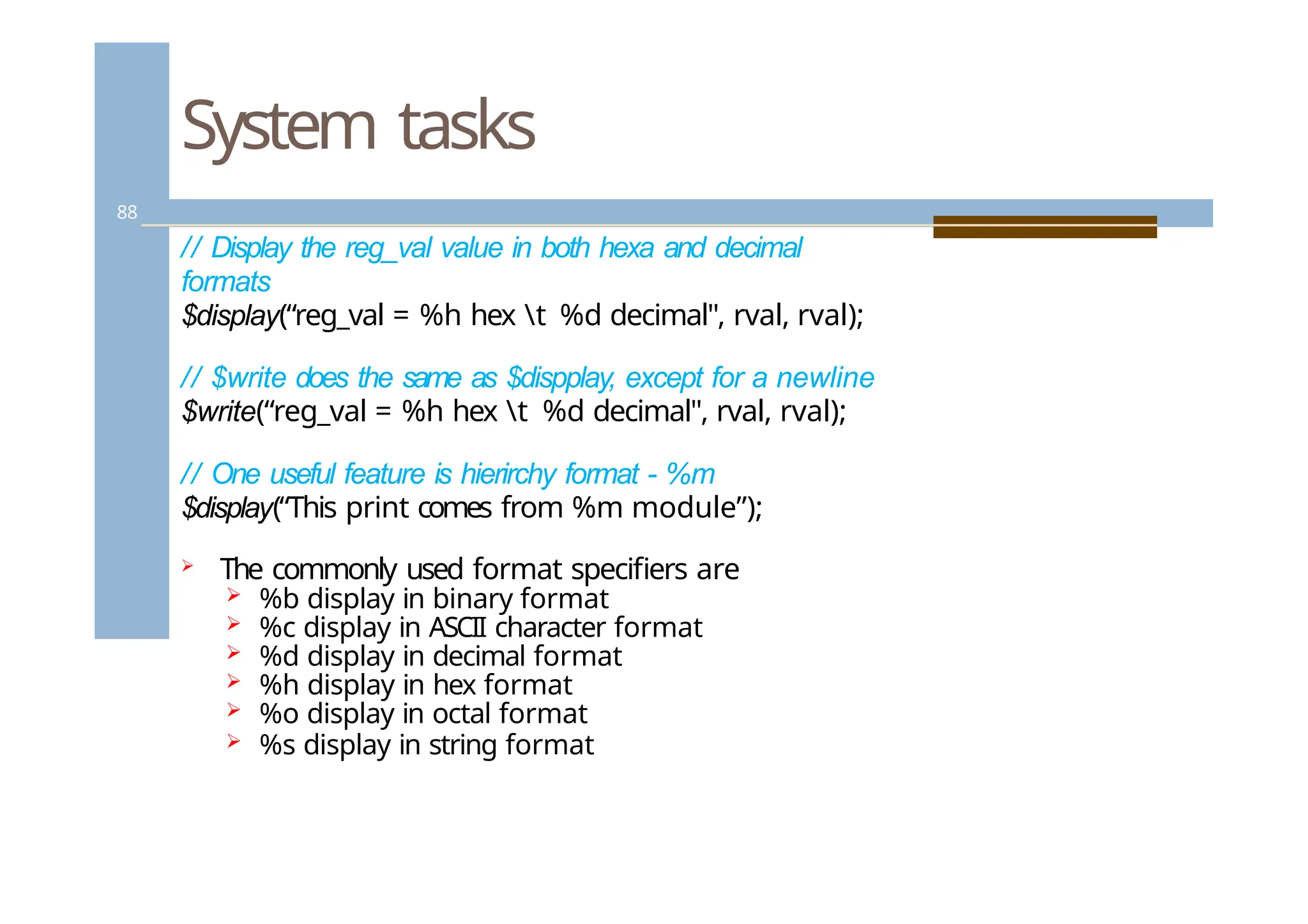
// Display the reg_val value in both hexa and decimal
formats
$display(“reg_val = %h hex t %d decimal", rval, rval);
// $write does the same as $dispplay, except for a newline
$write(“reg_val = %h hex t %d decimal", rval, rval);
// One useful feature is hierirchy format - %m
$display(“This print comes from %m module”);
 The commonly used format specifiers are
 %b display in binary format
 %c display in ASCII character format
 %d display in decimal format
 %h display in hex format
 %o display in octal format
 %s display in string format

88. System tasks
89
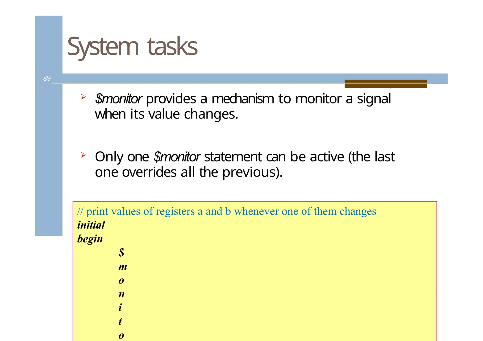
 $monitor provides a mechanism to monitor a signal
when its value changes.
 Only one $monitor statement can be active (the last
one overrides all the previous).
// print values of registers a and b whenever one of them changes
initial
begin
$
m
o
n
i
t
o

89. System tasks
90
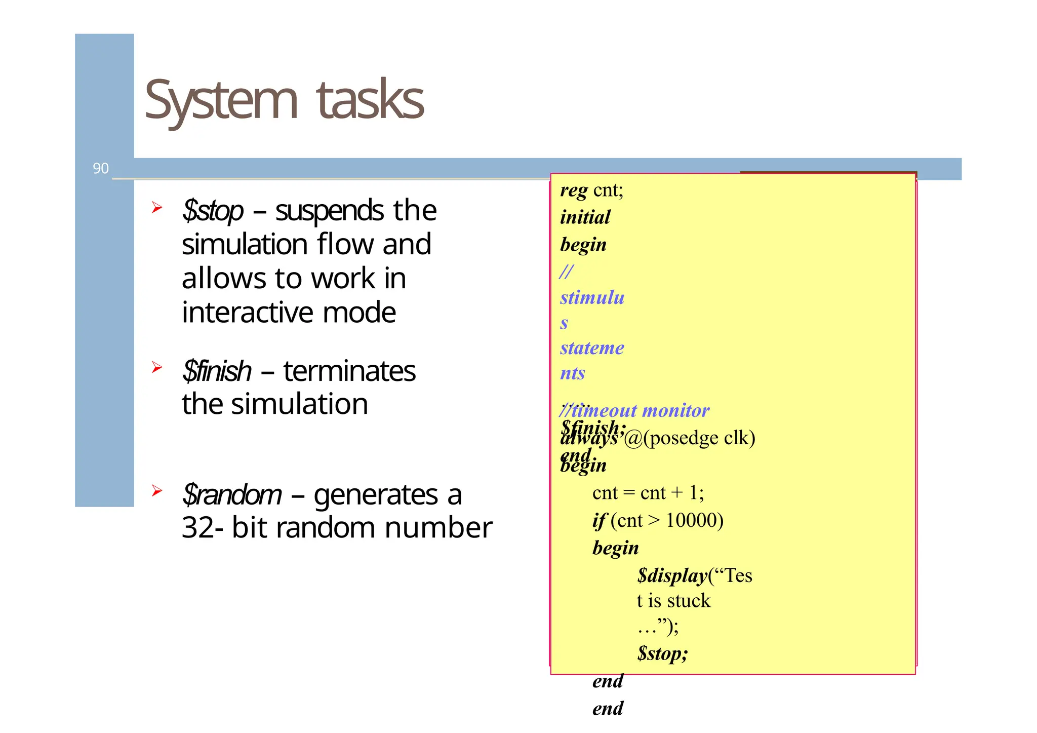
 $stop – suspends the
simulation flow and
allows to work in
interactive mode
 $finish – terminates
the simulation
 $random – generates a
32- bit random number
reg cnt;
initial
begin
//
stimulu
s
stateme
nts
…..
$finish;
end
//timeout monitor
always @(posedge clk)
begin
cnt = cnt + 1;
if (cnt > 10000)
begin
$display(“Tes
t is stuck
…”);
$stop;
end
end

90. System tasks - Value Change Dump
(VCD) File Tasks
91
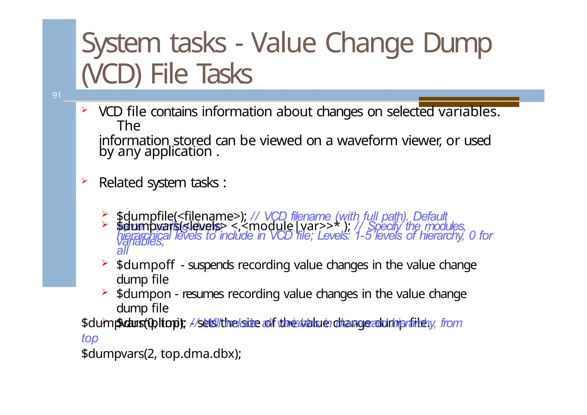
 VCD file contains information about changes on selected variables.
The
information stored can be viewed on a waveform viewer
, or used
by any application .
 Related system tasks :
 $dumpfile(<filename>); // VCD filename (with full path). Default
name : verilog.dump
 $dumpvars(<levels> <,<module|var>>* ); // Specify the modules,
variables,
hierarchical levels to include in VCD file; Levels: 1-5 levels of hierarchy, 0 for
all
 $dumpoff - suspends recording value changes in the value change
dump file
 $dumpon - resumes recording value changes in the value change
dump file
 $dumplimit - sets the size of the value change dump file.
$dumpvars(0, top); // Will include all variables in downward hierarchy, from
top
$dumpvars(2, top.dma.dbx);

91. Basic testbench
92
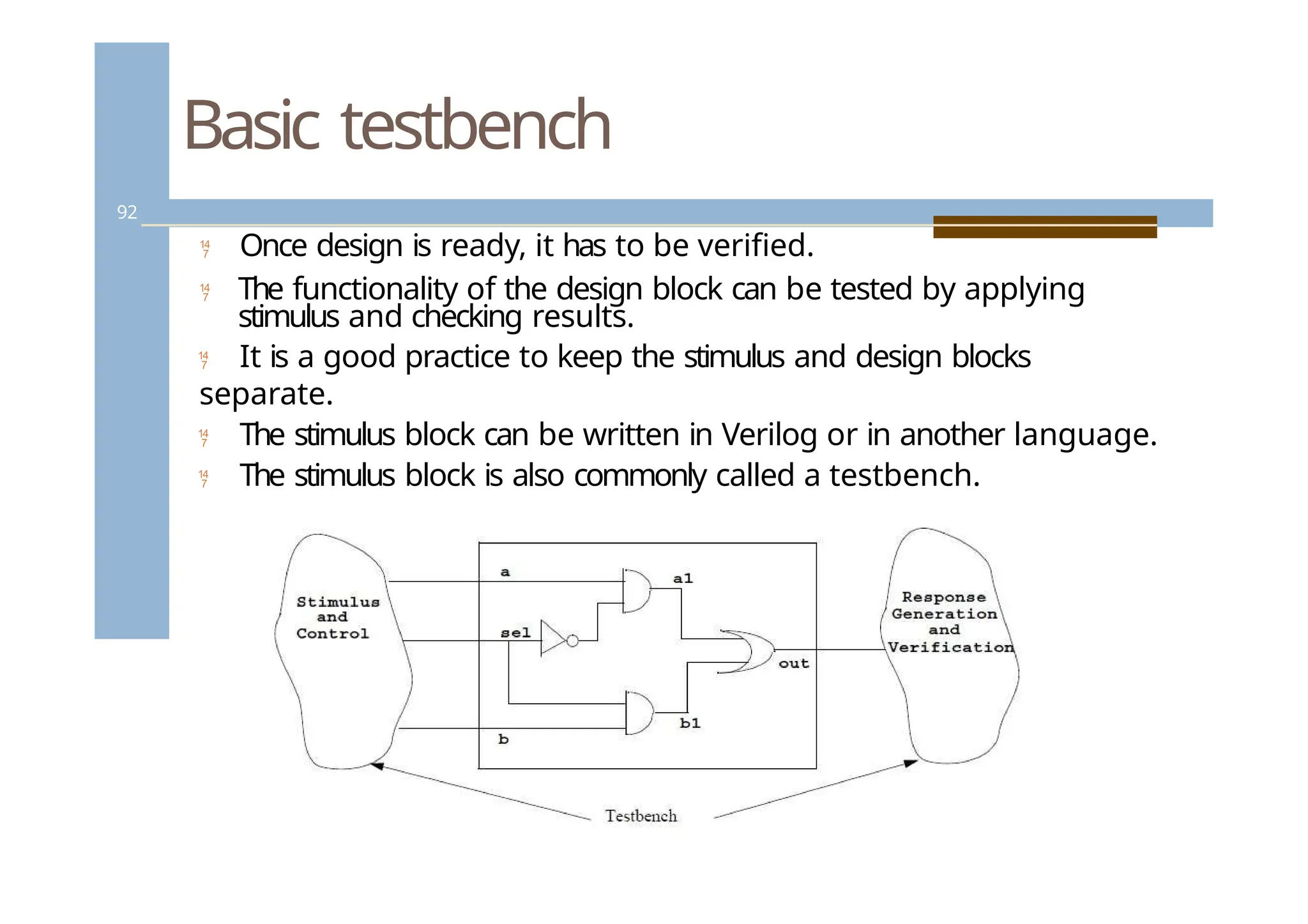
 Once design is ready, it has to be verified.
 The functionality of the design block can be tested by applying
stimulus and checking results.
 It is a good practice to keep the stimulus and design blocks
separate.
 The stimulus block can be written in Verilog or in another language.
 The stimulus block is also commonly called a testbench.