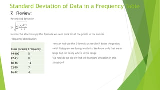
The document explains how to calculate the standard deviation for data presented in a frequency table, highlighting the limitations of using basic formulas due to lack of detailed data. It provides a specific formula for frequency distributions and includes a worked example with class ranges and calculations. The final computed standard deviation for the given data set is approximately 8.43.

1. Understanding Statistics
Standard Deviation of Data in a Frequency Table

2. Standard Deviation of Data in a Frequency Table
x̅̅̅̅ Review:
Review Std deviation
S=
𝑋𝑖−x̅̅̅̅ 2
𝑛−1
In order be able to apply this formula we need data for all the points in the sample
Frequency distribution:
- we can not use the S formula as we don’t know the grades
- with histogram we lose granularity. We know only that are in
range but not really where in the range
- So how do we do we find the Standard deviation in this
situation?
Class (Grade) Frequency
94-100 5
87-93 8
80-86 12
73-79 7
66-72 4

3. Standard Deviation of Data in a Frequency Table
It can be proven for frequency distribution that :
S=
[𝑛 𝑓∗𝑥2
− 𝑓∗𝑥 2
]
𝑛(𝑛−1)
n - sample size
f – frequency
X – midpoint of the class
n=36
One way to solve that equation (other than algorithms or specialised programing language like R) is to create additional rows
in the initial table
S=
36 253989 − 3009 2
36(36−1)
= 8.43
Class (Grade) Frequency Class midpoint (f*X) f*x2
94-100 5 97 485 47045
87-93 8 90 720 64800
80-86 12 83 996 82668
73-79 7 76 532 40432
66-72 4 69 276 19044
3009 253989
∑1 = 3009
∑2= 253989