The document presents a study on Unbiased Markov Chain Monte Carlo (MCMC) methods, focusing on a proposed methodology involving coupled chains to achieve unbiased estimators for Bayesian inference. It discusses the implementation of MCMC algorithms, specifically the Metropolis-Hastings method, and highlights the importance of maximizing coupling to improve efficiency and reduce bias. Additionally, the paper includes applications in neuroscience, showcasing its relevance in estimating parameters using particle filters and controlled sequential Monte Carlo methods.

1. Unbiased Markov chain Monte Carlo
Jeremy Heng
Information Systems, Decision Sciences and Statistics (IDS)
Department, ESSEC
Joint work with Pierre Jacob
Department of Statistics, Harvard University
ESSEC workshop on Monte Carlo Methods and Approximate
Dynamic Programming with Applications in Finance
18 October 2019
Jeremy Heng Unbiased MCMC 1/ 34

2. Setting
• Target distribution
⇡(dx) = ⇡(x)dx, x 2 Rd
• For Bayesian inference, target is the posterior distribution of
parameters x given data y
⇡(x) = p(x|y) / p(x)
|{z}
prior
p(y|x)
| {z }
likelihood
• Objective: compute expectation
E⇡ [h(X)] =
Z
Rd
h(x)⇡(x)dx
for some test function h : Rd ! R
• Monte Carlo method: sample X0, . . . , XT ⇠ ⇡ and compute
1
T + 1
TX
t=0
h(Xt) ! E⇡ [h(X)] as T ! 1
Jeremy Heng Unbiased MCMC 2/ 34

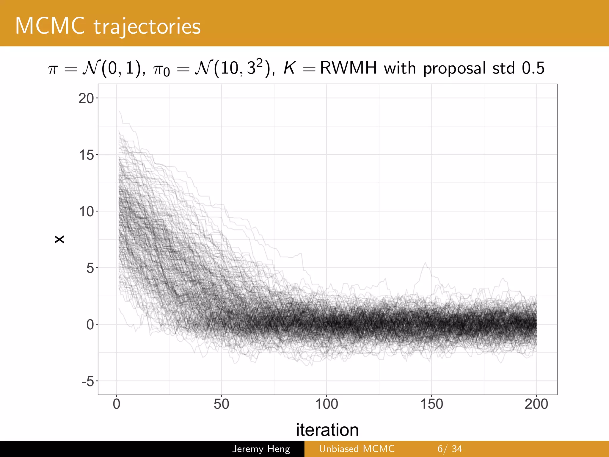
3. Markov chain Monte Carlo (MCMC)
• MCMC algorithm defines ⇡-invariant Markov kernel K
• Initialize X0 ⇠ ⇡0 6= ⇡ and iterate
Xt ⇠ K(Xt 1, ·) for t = 1, . . . , T
• Compute
1
T b + 1
TX
t=b
h(Xt) ! E⇡ [h(X)] as T ! 1
where b 0 iterations are discarded as burn-in
• Estimator is biased for any fixed b and T since ⇡0 6= ⇡
• Therefore averaging over independent copies does not
provide a consistent estimator of E⇡ [h(X)] as copies ! 1
Jeremy Heng Unbiased MCMC 3/ 34

4. Metropolis–Hastings (kernel K)
At iteration t, Markov chain at state Xt
1 Propose X? ⇠ q(Xt, ·), e.g. random-walk X? ⇠ N(Xt, 2Id ),
2 Sample U ⇠ U([0, 1])
3 If
U  min
⇢
1,
⇡(X?)q(X?, Xt)
⇡(Xt)q(Xt, X?)
,
set Xt+1 = X?, otherwise set Xt+1 = Xt
Jeremy Heng Unbiased MCMC 4/ 34

5. MCMC trajectory
⇡ = N(0, 1), ⇡0 = N(10, 32), K = RWMH with proposal std 0.5
Jeremy Heng Unbiased MCMC 5/ 34

6. MCMC trajectories
⇡ = N(0, 1), ⇡0 = N(10, 32), K = RWMH with proposal std 0.5
Jeremy Heng Unbiased MCMC 6/ 34

7. MCMC marginal distributions
⇡ = N(0, 1), ⇡0 = N(10, 32), K = RWMH with proposal std 0.5
Jeremy Heng Unbiased MCMC 7/ 34

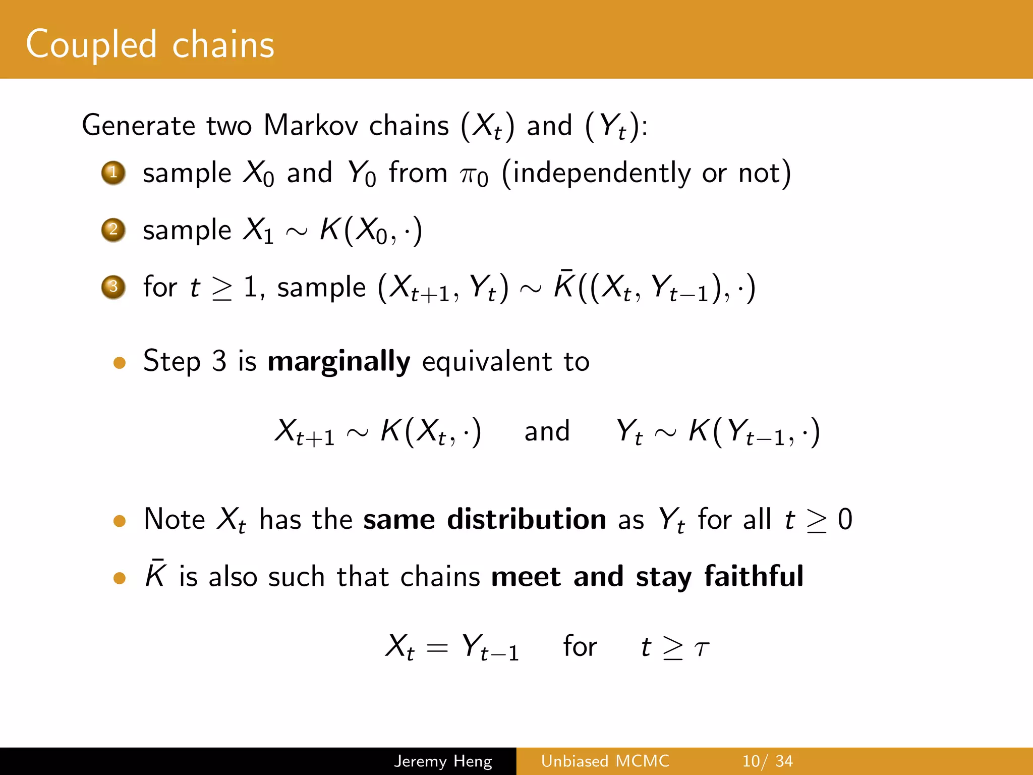
8. Proposed methodology
• Each processor runs two
coupled chains X = (Xt) and
Y = (Yt)
• Terminates at some random
time which involves their
meeting time
• Returns unbiased estimator
Hk:m of E⇡ [h(X)]
• Average over independent
copies to consistently estimate
E⇡ [h(X)] as copies ! 1
• E ciency depends on
expected compute cost and
variance of Hk:m
Parallel MCMC
processors
1
Jeremy Heng Unbiased MCMC 8/ 34

9. Parallel computing
Glynn & Heidelberger. Bias Properties of Budget Constrained
Simulations (1990)
Jeremy Heng Unbiased MCMC 9/ 34

10. Coupled chains
Generate two Markov chains (Xt) and (Yt):
1 sample X0 and Y0 from ⇡0 (independently or not)
2 sample X1 ⇠ K(X0, ·)
3 for t 1, sample (Xt+1, Yt) ⇠ ¯K((Xt, Yt 1), ·)
• Step 3 is marginally equivalent to
Xt+1 ⇠ K(Xt, ·) and Yt ⇠ K(Yt 1, ·)
• Note Xt has the same distribution as Yt for all t 0
• ¯K is also such that chains meet and stay faithful
Xt = Yt 1 for t ⌧
Jeremy Heng Unbiased MCMC 10/ 34

11. Debiasing idea
Glynn & Rhee. Exact estimation for Markov chain equilibrium
expectations (2014)
• Writing limit as telescopic sum (starting from k 0)
E⇡ [h(X)] = lim
t!1
E [h(Xt)] = E [h(Xk)]+
1X
t=k+1
E [h(Xt) h(Xt 1)]
• Since Xt has the same distribution as Yt for all t 0
E⇡ [h(X)] = E [h(Xk)] +
1X
t=k+1
E [h(Xt) h(Yt 1)]
• If interchanging summation and expectation is valid
E⇡ [h(X)] = E
"
h(Xk) +
1X
t=k+1
h(Xt) h(Yt 1)
#
Jeremy Heng Unbiased MCMC 11/ 34

12. Debiasing idea
• Truncate infinity sum since Xt = Yt 1 for t ⌧
E⇡ [h(X)] = E
"
h(Xk) +
⌧ 1X
t=k+1
h(Xt) h(Yt 1)
#
with the convention
P⌧ 1
t=k+1{·} = 0 if k + 1 > ⌧ 1
• Unbiased estimator for any k 0
Hk(X, Y ) = h(Xk) +
⌧ 1X
t=k+1
{h(Xt) h(Yt 1)}
• First term h(Xk) is biased; second term corrects for bias
Jeremy Heng Unbiased MCMC 12/ 34

13. Unbiased estimators
Jacob et al. Unbiased Markov chain Monte Carlo with couplings
(2019)
For any k 0, Hk(X, Y ) is an unbiased estimator of E⇡ [h(X)],
with finite variance and expected cost if
1 Convergence of marginal chain:
lim
t!1
E [h(Xt)] = E⇡ [h(X)] and sup
t 0
E|h(Xt)|2+
< 1, > 0
2 Meeting time ⌧ = inf{t 1 : Xt = Yt 1} has geometric or
polynomial tails:
3 Faithfulness: Xt = Yt 1 for t ⌧
Jeremy Heng Unbiased MCMC 13/ 34

14. Time-averaged estimators
• Since Hk(X, Y ) is unbiased for all k 0, the time-averaged
estimator
Hk:m(X, Y ) =
1
m k + 1
mX
t=k
Ht(X, Y ) for any k  m
is also unbiased
• Rewrite estimator as
1
m k + 1
mX
t=k
h(Xt) +
⌧ 1X
t=k+1
min
✓
1,
t k
m k + 1
◆
{h(Xt) h(Yt 1)}
• First term is standard MCMC average; second term is bias
correction (zero if k + 1 > ⌧ 1)
Jeremy Heng Unbiased MCMC 14/ 34

15. Time-averaged estimators
• Bias removal leads to variance inflation
• Variance inflation can be mitigated by increasing k and m
• If ⌧ ⌧ k ⌧ m, asymptotic ine ciency of Hk:m(X, Y ) is
approximately the asymptotic variance of marginal chain
Glynn & Whitt, The asymptotic e ciency of simulation
estimators (1992)
Jeremy Heng Unbiased MCMC 15/ 34

16. Maximal coupling
• A key tool to simulate chains that meet is a maximal
coupling between two distributions p(x) and q(y) on Rd
• A maximal coupling c(x, y) is a joint distribution on Rd ⇥ Rd
such that:
(i) (X, Y ) ⇠ c implies X ⇠ p and Y ⇠ q
(ii) P(X = Y ) is maximized
• There is an algorithm to sample from a maximal coupling if
(i) sampling from p and q is possible
(ii) evaluating the densities of p and q is tractable
Thorisson. Coupling, stationarity, and regeneration (2000)
Jeremy Heng Unbiased MCMC 16/ 34

17. Independent coupling of Gamma and Normal
Jeremy Heng Unbiased MCMC 17/ 34

18. Maximal coupling of Gamma and Normal
Jeremy Heng Unbiased MCMC 18/ 34

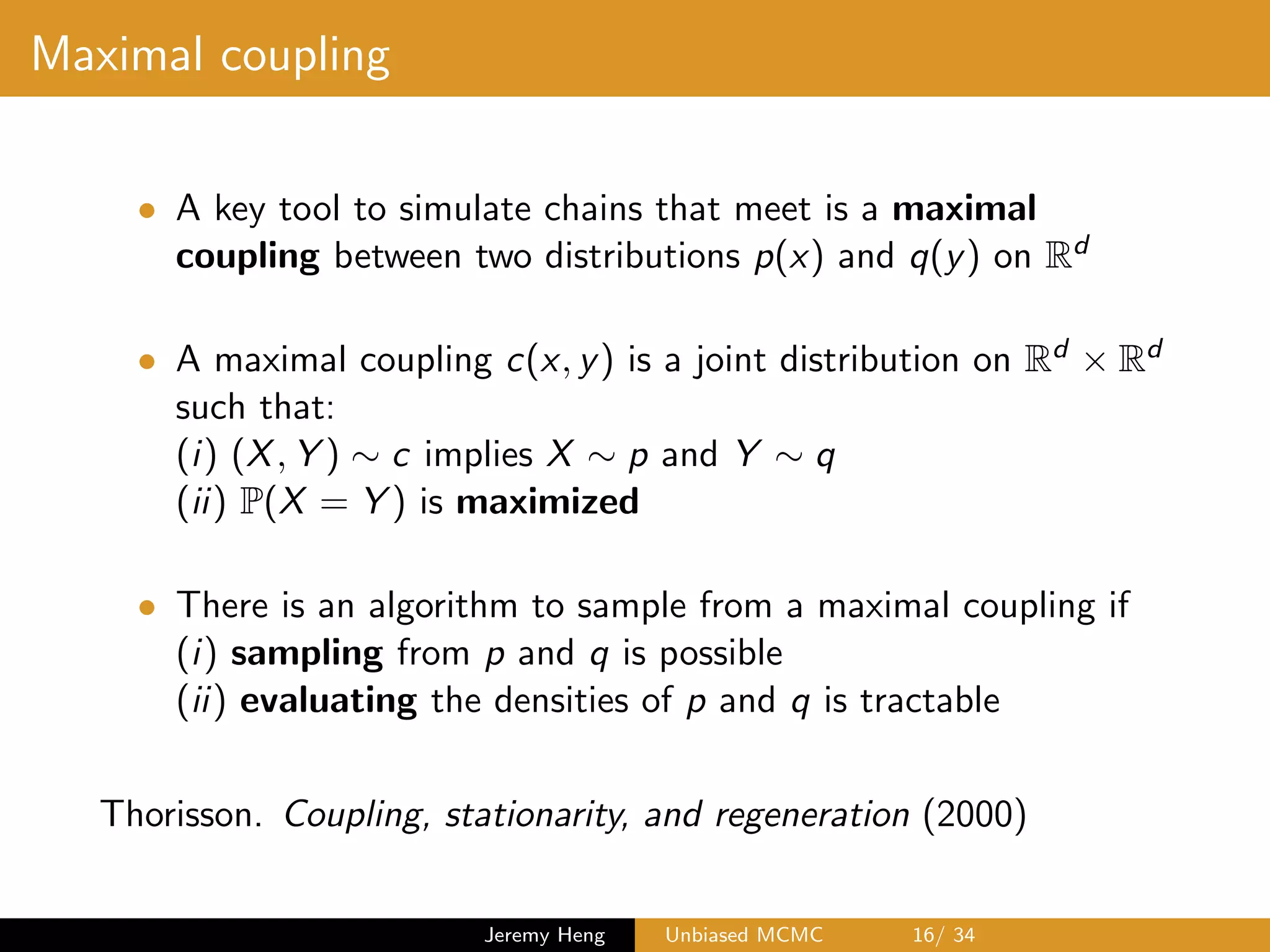
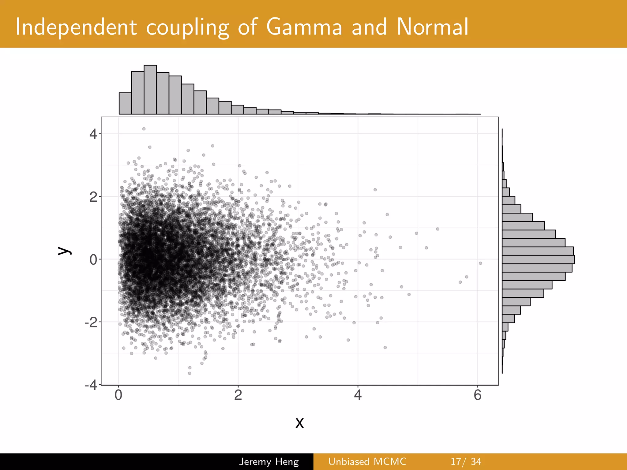
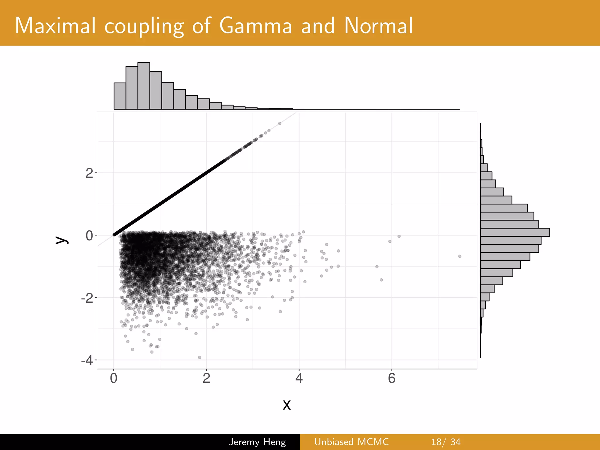
19. Maximal coupling: algorithm
Sampling (X, Y ) from maximal coupling of p and q
1 Sample X ⇠ p and U ⇠ U([0, 1])
If U  q(X)/p(X), output (X, X)
2 Otherwise, sample Y ? ⇠ q and
U? ⇠ U([0, 1])
until U? > p(Y ?)/q(Y ?), and
output (X, Y ?)
Normal(0,1)
Gamma(2,2)
0.0
0.2
0.4
0.6
0.8
−5.0 −2.5 0.0 2.5 5.0
space
density
Jeremy Heng Unbiased MCMC 19/ 34

20. Maximal coupling: algorithm
• Step 1 samples from overlap
min{p(x), q(x)}
• Maximality follows from coupling
inequality
P(X = Y ) =
Z
Rd
min{p(x), q(x)}dx
= 1 TV(p, q)
• Expected cost does not depend
on p and q (but variance does!)
Normal(0,1)
Gamma(2,2)
0.0
0.2
0.4
0.6
0.8
−5.0 −2.5 0.0 2.5 5.0
space
density
Jeremy Heng Unbiased MCMC 20/ 34

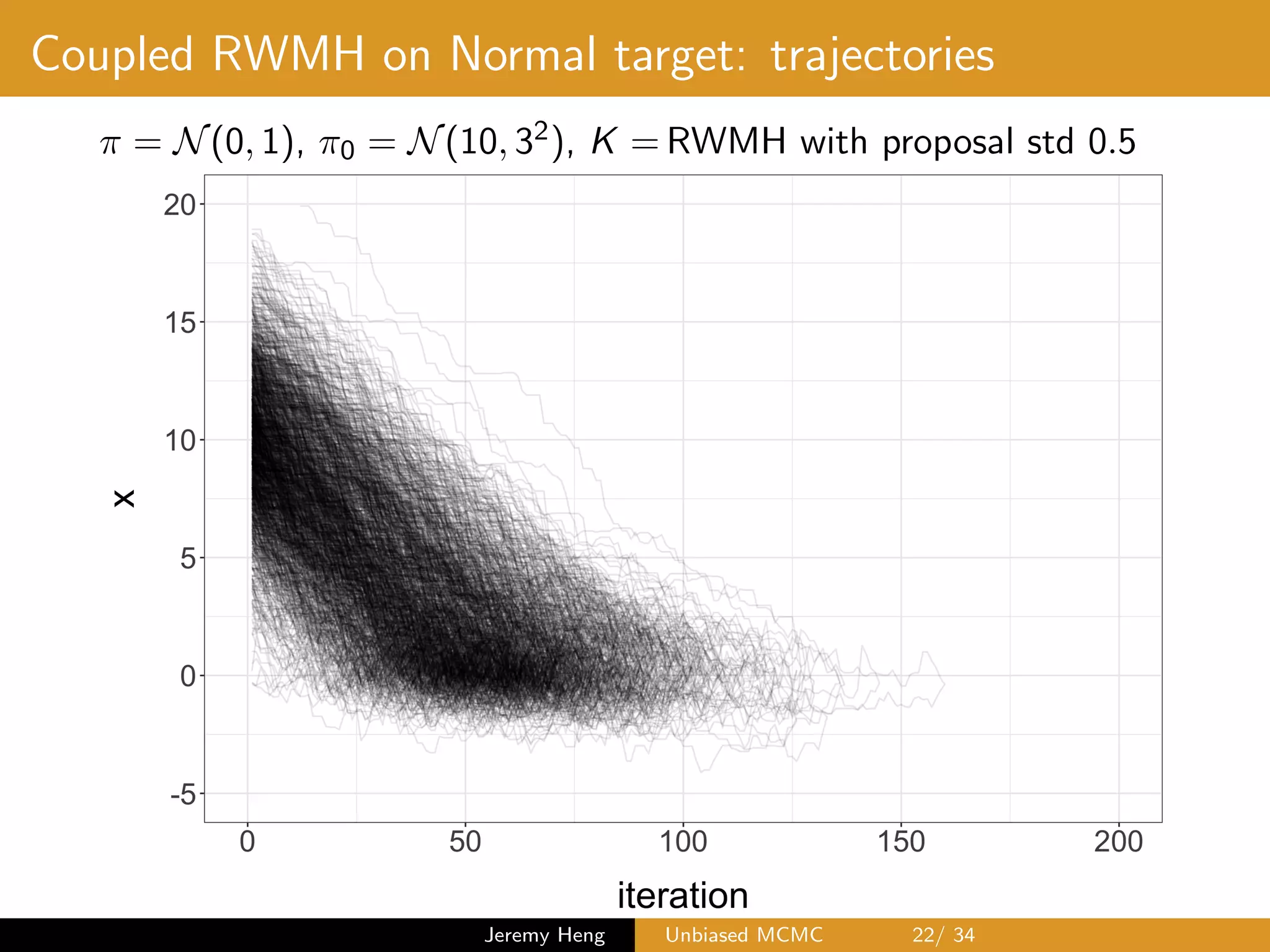
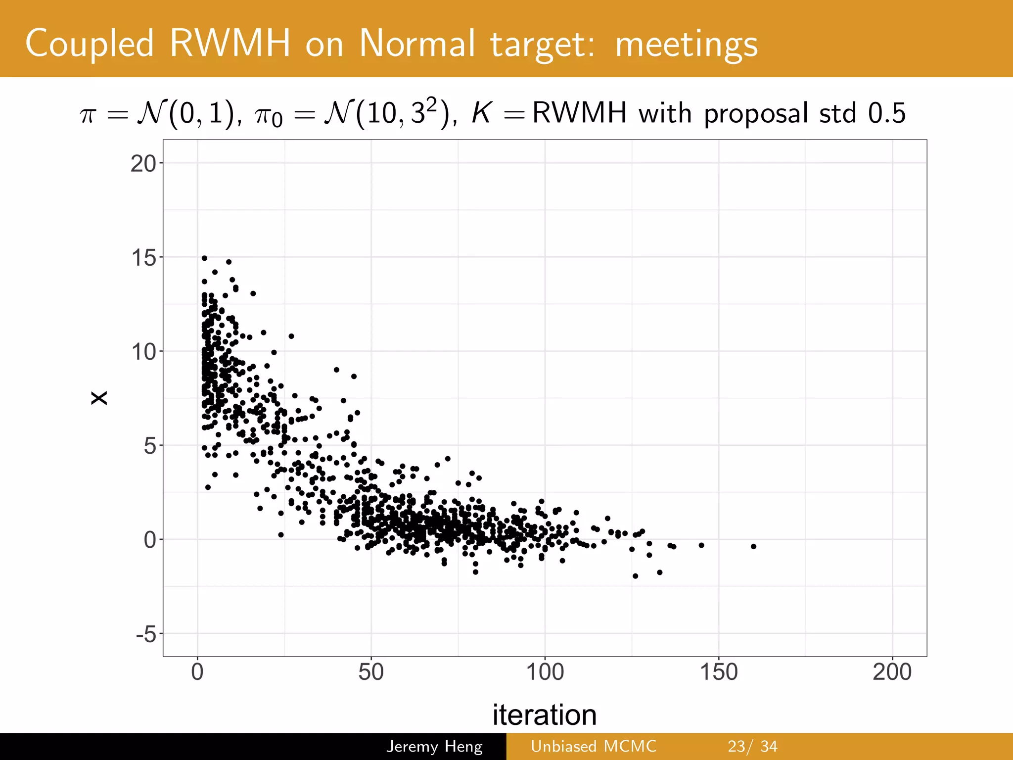
21. Coupled Metropolis–Hastings (kernel ¯K)
At iteration t, two Markov chains at states Xt and Yt 1
1 Propose (X?, Y ?) from maximal coupling of q(Xt, ·) and
q(Yt 1, ·)
2 Sample U ⇠ U([0, 1])
3 If
U  min
⇢
1,
⇡(X?)q(X?, Xt)
⇡(Xt)q(Xt, X?)
,
set Xt+1 = X?, otherwise set Xt+1 = Xt
If
U  min
⇢
1,
⇡(Y ?)q(Y ?, Yt 1)
⇡(Yt 1)q(Yt 1, Y ?)
,
set Yt = Y ?, otherwise set Yt = Yt 1
Jeremy Heng Unbiased MCMC 21/ 34

22. Coupled RWMH on Normal target: trajectories
⇡ = N(0, 1), ⇡0 = N(10, 32), K = RWMH with proposal std 0.5
Jeremy Heng Unbiased MCMC 22/ 34

23. Coupled RWMH on Normal target: meetings
⇡ = N(0, 1), ⇡0 = N(10, 32), K = RWMH with proposal std 0.5
Jeremy Heng Unbiased MCMC 23/ 34

24. Coupled RWMH on Normal target: meeting times
⇡ = N(0, 1), ⇡0 = N(10, 32), K = RWMH with proposal std 0.5
0.000
0.005
0.010
0.015
0 50 100 150 200
meeting time
density
Jeremy Heng Unbiased MCMC 24/ 34

25. Neuroscience example
• Joint work with Demba Ba, Harvard School of Engineering
• 3000 measurements yt 2 {0, . . . , 50} collected from a
neuroscience experiment (Temereanca et al., 2008)
Temereanca, Brown & Simons, Rapid changes in thalamic firing
synchrony during repetitive whisker stimulation (2008)
Jeremy Heng Unbiased MCMC 25/ 34

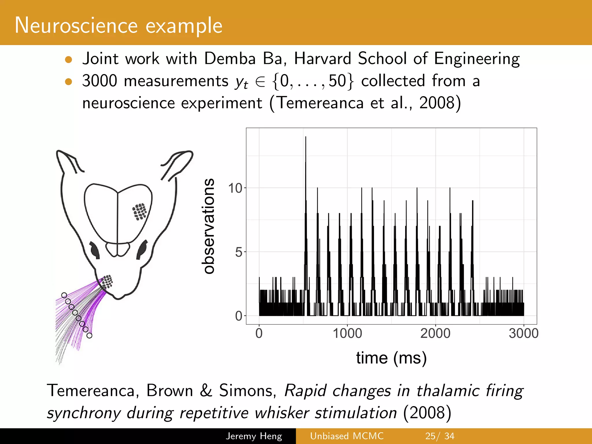
26. Neuroscience example
• Observation model
Yt|Xt ⇠ Binomial 50, (1 + exp( Xt)) 1
• Latent Markov chain
X0 ⇠ N(0, 1), Xt|Xt 1 ⇠ N(aXt 1, 2
X )
• Unknown parameters are (a, 2
X ) 2 [0, 1] ⇥ (0, 1)
• Particle marginal Metropolis–Hastings (PMMH) to sample
p(a, 2
X |y0:T ) / p(a, 2
X )p(y0:T |a, 2
X )
and particle filters to unbiasedly estimate the likelihood
p(y0:T |a, 2
X ) =
Z
RT+1
p(x0:T , y0:T |a, 2
X ) dx0:T
Andrieu, Doucet & Holenstein. Particle Markov chain Monte
Carlo methods (2010)
Jeremy Heng Unbiased MCMC 26/ 34

27. Likelihood estimation
• Bootstrap particle filter (BPF) moves N particles using
p(xt|xt 1) without taking observations into account
• Likelihood estimator has high variance for practical values of
N
• Controlled sequential Monte Carlo (cSMC) moves particles
using an approximation of
p(xt|xt 1, yt:T ) / p(xt|xt 1)p(yt:T |xt)
• As backward information filter satisfies
p(yt:T |xt) = p(yt|xt)
Z
R
p(yt+1:T |xt+1)p(xt+1|xt) dxt+1
we exploit approximate dynamic programming methods
Heng, Bishop, Deligiannidis & Doucet. Controlled sequential
Monte Carlo (2017).
Jeremy Heng Unbiased MCMC 27/ 34

28. BPF vs cSMC
Relative variance of log-likelihood estimator with a = 0.99
0.05 0.1 0.15 0.2
-9.5
-9
-8.5
-8
-7.5
-7
-6.5
-6
-5.5
Jeremy Heng Unbiased MCMC 28/ 34

29. Posterior estimation
Log-posterior density estimated using cSMC with N = 128
particles and I = 3 iterations (⇡ 1 second per parameter)
Jeremy Heng Unbiased MCMC 29/ 34

30. Choice of proposal standard deviation
Meeting times of coupled PMMH chains initialized independently
from ⇡0 = U([0, 1]2)
Figure: Right plot uses 5 times the proposal standard deviation of left plot
Jeremy Heng Unbiased MCMC 30/ 34

31. Choice of proposal standard deviation
Traces of chains for largest meeting time of 21,570 (with smaller
proposal std)
0.00
0.25
0.50
0.75
1.00
0 5000 10000 15000 20000
iteration
a
0
1
2
3
0 5000 10000 15000 20000
iteration
σX
2
Therefore larger proposal std allows chains to escape region of
high variance of the likelihood estimator
Jeremy Heng Unbiased MCMC 31/ 34

32. Choice of particle filter
Meeting times of coupled PMMH chains initialized independently
from ⇡0 = U([0, 1]2)
Figure: cSMC (left) and BPF (right) with N = 4, 096 to match compute
time
Jeremy Heng Unbiased MCMC 32/ 34

33. Unbiased estimation of marginal posteriors
Choosing k = 1, 000 and m = 10k results in relative ine ciency
of 1.07 and compute time of < 3 hours
Figure: Histogram of parameters using unbiased estimation against long
run of PMMH (red)
Jeremy Heng Unbiased MCMC 33/ 34

34. References
• Jacob, O’Leary & Atchad´e. Unbiased Markov chain Monte
Carlo with couplings. JRSSB (with discussion), 2019.
• Middleton, Deligiannidis, Doucet & Jacob. Unbiased Markov
chain Monte Carlo for intractable target distributions. 2018.
• Heng & Jacob. Unbiased Hamiltonian Monte Carlo with
couplings. Biometrika, 2019.
• Jacob, Lindsten, Sch¨on. Smoothing with Couplings of
Conditional Particle Filters. JASA, 2018.
Jeremy Heng Unbiased MCMC 34/ 34