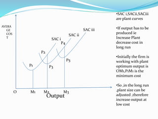
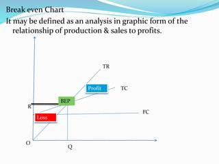
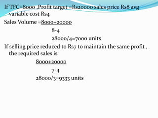
Cost and production analysis - Cost concepts – Cost and output relationship - cost control – Short run and Long run - cost functions - production functions – Break-even analysis - Economies scale of production.

1. MANAGERIAL ECONOMICS
UNIT -3
Prepared By
Ms.Jissy.C
Assistant Professor

2. UNIT – III
 Cost and production analysis - Cost concepts – Cost and
output relationship - cost control – Short run and Long run -
cost functions - production functions – Break-even analysis -
Economies scale of production.

3. Cost of production
The term Cost of production means the expenses incurred
in the production of a commodity
This refers to the total amount of money spent on the
production of the commodity
Definition: In economics, the Cost Analysis refers to the
measure of the cost – output relationship, i.e. the
economists are concerned with determining the cost
incurred in hiring the inputs and how well these can be re-
arranged to increase the productivity (output) of the firm.

4. There are several cost concepts relevant to the business
operations and decisions and for the convenience of
understanding these can be grouped under two
overlapping categories:
Cost Concepts Used for Accounting Purposes
Analytical Cost Concepts Used for Economic Analysis
of Business Activities

5. Cost Concepts Used for Accounting Purposes:
Generally, the accountants use these cost concepts to study
the financial position of the firm. They are concerned with
arranging the finances of the firm and therefore keep a
track of the assets and liabilities of the firm. The
accounting costs are used for taxation purposes and
calculating the profit and loss of the firm. These are:
Opportunity Cost
Business Cost
Full Cost
Explicit cost
Implicit Cost
Out-of-Pocket Cost
Book Cost

6. Analytical Cost Concepts Used for Economic Analysis
of Business Activities:
These cost concepts are used by the economists to analyze
the likely cost of production in the future. They are
concerned with how the cost of production can be
managed or how the input and output can be re-arranged
such that the overall profitability of the firm gets
improved. These costs are:
Fixed Cost Long-run Cost
Variable cost Incremental Cost
Total Cost Historical Cost
Average Cost Replacement Cost
Marginal Cost Private Cost
Short-run Cost Social Cost

7. Total Cost, Average Cost, Marginal Cost
Total Cost(TC)
Total money expenses incurred for buying the inputs
required to produce a commodity
TC=TFC + TVC
TC=Total cost, TFC =Total Fixed Cost ,TVC=Total Variable Cost.
TC
TVC
TFC
Output
Cost
Y
X
•TFC is horizontal as,
whatever be the output TFC is
Same
•TVC Starts from origin ie, if
output is O,TVC is also Zero.
•TC=TFC + TVC ,so ot starts
from Y axis

8. Average Cost(AC)
Average cost is the cost per unit of output
AC=TC/Q ,AC =Average Cost , TC=Total Cost ,Q= Output
Produced
If TC =100; Q= 10; then AC=100/10= Rs 10/-
AC=AFC + AVC

9. Marginal Cost:-
Marginal Cost may be defined as the addittion made to the
total cost by the production of one additional unit of
output.
MC= TC/ Q,
TC-Change in total cost
Q-Change in Output

10. COST-OUTPUT Relation
Cost Functions:-
The relation between cost & output is known as cost
function.
Types of Cost Function
1.Short run Cost Function
2.Long run Cost Function
Short run cost output relationship
Short run, only some inputs are variable & other inputs are
held constant.
To Increase or Decrease output, the variable inputs have to
be Increased or Decreased.

11. Short Run Production & Cost dataOut Put TFC TVC TC AFC AVC AC MC
0 1000 0 1000 - - - -
1 1000 200 1200 1000 200 1200 200
2 1000 367 1367 500 184 684 167
3 1000 510 1510 333 170 503 143
4 1000 677 1677 250 169 419 167
5 1000 877 1877 200 175 375 200
6 1000 1127 2127 167 188 355 250
7 1000 1460 2460 143 209 352 333
8 1000
1
2460
2
3460
3
125
4
307
5
432
6
1000
7

12.  Where, TC=TFC +TVC
AFC=TFC/Output
AVC=TVC/Output
AC=AFC + AVC
MC=Difference of total Cost
Relationship among AVC, AC,MC can be explained with
the following figure:-

13. AFC
AVC
AC
MC
L
OUTPUT
COST

14.  AFC falls as output rises
 AC first falls & then rises
 AVC first falls & then rises
 AVC rises before AC rises
 L least cost output
 MC cuts AVC & AC at their minimum Points.

15. Long run Cost output relationship
 In Long-run ,all factors are variable
 If output has to be increased ,new building have to be
acquired or hired ,new machinery can be increased etc
 Long run cost of production is the least possible cost of
production of producing a given level of output when all
inputs are variable.
Long run Average Cost(LRAV) =LTC/Q
LTC= Long run total cost ; Q=Output

16. Output
AVERA
GE
COS
T
SAC i
SAC ii
SAC iii
O M1 M2 M3
P1
P2
P4
P3
P5
•SAC i,SACii,SACiii
are plant curves
•If output has to be
produced ie
Increase Plant
decrease cost in
long run
•Initially the firm is
working with plant
optimum output is
OM1,P1M1 is the
minimum cost
•So ,in the long run
,plant size can be
adjusted ,therefore
increase output at
low cost

17. Break-Even Analysis
 A breakeven analysis is used to determine how much sales
volume your business needs to start making a profit.
 The breakeven analysis is especially useful when you're
developing a pricing strategy, either as part of a marketing plan
or a business plan.
 The break-even point (BEP) in economics, business—and
specifically cost accounting—is the point at which total cost and
total revenue are equal, i.e. "even". There is no net loss or gain,
and one has "broken even", though opportunity costs have been
paid and capital has received the risk-adjusted, expected return.
In short, all costs that must be paid are paid, and there is
neither profit or loss.
 Total cost = Total revenue = B.E.P. INTRODUCTION

18. Break even Chart
It may be defined as an analysis in graphic form of the
relationship of production & sales to profits.
O
Q
R
TR
TCProfit
Loss
BEP
FC

19.  The horizontal axis shows output & the vertical axis
indicates costs & revenue.
 Both TC & TR curves are shown as linear.
 TR curve is linear because of the assumption of constant
variable cost.
 TR Curve is drawn as straight line from the origin because
every unit of output contributes constant amount to total
revenue
 TC curve is a straight line starting from Y axis because total
cost includes fixed & variable costs.
 The BEP is point is the point of intersection between TR
and TC curve. Below the BEP ,total costs are more than
total revenue and the firm would suffer a loss. Above the
BEP ,total revenue exceeds total cost & the firm and the
firm would be making profits.

20. Calculation of the BEP
BEP may also be analyzed in terms of volume of output.
The BEP is the number of units of the commodity that
should be sold to earn enough revenue just to cover all the
expenses without incurring a loss

21. Table ,Total Revenue,Total Cost & BEP
Selling price=R 4 per unit
Output in
units
Total Revenue Total Fixed
Cost
Total variable
cost
Total cost
0 0 150 0 150
50 200 150 150 300
100 400 150 300 450
150 600 150 450 600
200 800 150 600 750
250 1000 150 750 900
300 1200 150 900 1050

22. When the output is zero ,the firm incurs only fixed cost. When
the output is 50, the total cost is Rs300.The total revenue is
Rs200.The firm incurs a loss of Rs 100.Similarily when the
output is 100,the firm incurs a loss of Rs50.At the level of output
150 units the total revenue is equal to total cost. At this level the
firm is working at a point where there is no profit or loss. This is
the BEP .From the level of output of 200 the firm is making
profit.
There is another way of finding out BEP in terms of physical
units of output. Instead of using total revenue and total cost ,we
can use average revenue & average cost.The BEP is the level of
output at which the price of the product (AR) covers the average
cost.The price should cover average variable cost and a portion
of average fixed cost.The excess of selling price over average
variable cost goes towards meeting some portion of the fixed
cost .This excess cost is called contribution margin.So the BEP
will be at a point where the total contribution margin is equal to
the total fixed cost.

23. BEP=Total Fixed cost/Contribution margin per unit
Contribution margin can be found out by deducting the
average variable cost from the selling so
BEP=Total fixed cost/Selling price-AVC
For eg,the total fixed cost is Rs.150 ,the selling price is Rs2 &
the average variable cost is Re1
BEP=150/2-1=150.
The BEP on the basis of formula comes to 150 units of output

24. Contribution Margin
Output
TR
TC
TVC
Fixed Cost
Variable CostLoss
Profit
O
BEP
Q
A
C
o
s
t
R
e
v
e
n
u
e
&
P
r
i
c
e
Break Even charts are often used to
determine the contribution margin.
Contribution margin is the difference
between receipts & margin expense

25. ASSUMPTIONS.
 It assumes that can be classified into fixed & variable cost .It
ignores semi-variable cost
 All revenue is perfectly variable with the physical volume of
production
 The volume of sales & the volume of production are equal
 The price of the product is assumed to be constant
 It assumes constant rate of increase in variable cost, thereby
giving rise to a linear total cost curve.
 Changes in input prices are ruled out.

26. Limitations
 The break even analysis assumes that the product are
given.
 The break-even analysis is static as it assumes a constant
relationship of output to costs & revenue.
 Break even analysis is an effective tool for the short run &
not an effective one for long run use.
 Break even analysis assumes that the cost –revenue –
volume relationship is linear. This is realistic only over
narrow ranges of output
 The break –even analysis is based on accounting data.

27. Use of Break-even Analysis
 Safety Margin
Safety margin refers to extent to which the firm can afford a decline insales
before it starts incuring loses.
Safety of margin=(Sale-BEP )/Sales X100
 Target Profit
Break even analysis may be used for determining the volume of sales
necessary to achieve a target profit
Target sales Volume= Fixed Cost + Target Profit
Contribution margin per unit
 Change in Price
 The formula for determining the new volume of slaes to maintain the same
profit with given reduction in price will be as follows:-
 New sales volume= Total fixed cost + Total profit
New selling price – Avg Variable cost

28. If TFC=8000 ,Profit target =Rs20000 sales price Rs8 avg
variable cost Rs4
Sales Volume =8000+20000
8-4
28000/4=7000 units
If selling price reduced to Rs7 to maintain the same profit ,
the required sales is
8000+20000
7-4
28000/3=9333 units

29.  Change in costs
The impact of an increase in variable cost is push up the
total cost while contribution margin declines. This decline
in the contribution margin will shift the break evev point
downwards & vice versa.
 Make or buy decision
Break even analysis also help to decide whether
components which are part of their finished should be
manufactured by themselves or brought from outside firm.
 Advertising Decision
The break even concept helps the management to know
about the circum stances under which the decision has to
be taken. Thus it help the management to decide about the
best promotion –mix policy

30. Cost control &cost reduction
 Cost Control
Cost control is an important perquisite for the successful
operation of a business. The competitive ability of the firm
depends upon the ability to produce the commodity at the
minimum cost .This involves cost consciousness on the
part of the firms .
 Cost control by management means a for search better
and more economical ways of completing each operation.
 it aims at keeping the costs down thereby increasing the
profitability & competence of the firm & making best use
of every rupee spent in producing a commodity.
 Cost control would mean a reduction in the percentage of
costs and in turn an increase in the percentage of profits.

31. Cost Control has two aspects:
Reduction in specific expenses
More efficient use of every rupee spent
Techniques of cost control:
Budgetary Control
Standard Costing
Budgetary Control
 It is concerned with the cost of running individual
departments within the company
 It is predetermined statement of management policy
during a given period which period which provides a
standard for comparison with the results actually
achieved

32. Standard Costing
 It is concerned with the cost of making particular products.
 It aims at establishing standards of performance & targets
cost which are to achieved under a given set of working
conditions
 It is a predetermined cost which determines what each
product or service should cost under given circumstances.
Other Techniques for cost reduction
 Marginal Costing
 Value Costing
 Work study
 Simplification & Variety reduction

33. Areas of control
 Materials
 Inventory Control
 Labour
 Overheads
Cost reduction & Cost control
 Cost reduction is confined to genuine saving in the cost of
manufacturing ,administration, distribution,& selling
brought about the elimination of wasteful and inessential
elements from the product design and form the techniques
& practices carried out in connection therewith.

34. Definition
Cost reduction has been defined by the institution of cost and
works accounts of London” the achievement of real and
permanent reductions in the unit of goods manufactured or
services rendered without impairing their suitability for the use
intended”
Essentials for the success of a cost reduction program
 Everyone in the firm should understand and recognise his
responsibility the corporations of every individual should be
insured by a careful dissemination of the objectives of the firm
in view and by increasing employees to identify their self
interest with the firms interest.
 Employees resistance to cost reduction program should be
minimised by disseminating complete information about the
proposed changes and also convincing the workers that is that
the changes are concerned with the problems faced by the
phone and that the workers would be the ultimate beneficiaries

35.  Cost reduction efforts should be continuously maintained
and effort should be made to explore new areas as a savings
could be achieved to the maximum
 There should be periodic meeting with the workers to
review the programs made towards cost reduction

36.  ECONOMICS OF SCALE
 Production may be carried on a small scale or on a large-
scale when a firm expands its size of production by
increasing all the factors, it’s a core certain advantages
known as Economics of production.
 Economics of Scale can de divide into Two Types
Internal Economics & External Economics
 Internal economics are those which are open to a single
factory or a simple form independently of the actions of
other firms. They result from an increase in the scale of
output of a firm and cannot be achieved word and less
output increases.
 External economics are those benefits which are shared in
by a numbers of firms or industries when the scale of
production in an industry or group of industries increases.

37.  Diseconomies of scale
 Diseconomies of scale arises ,which means that the
size of the firm grows so large that it becomes very
difficult to manage it .These diseconomies can be two
types:
 Internal diseconomies
 External diseconomies

38. Return to
scale
Economics of
Scale
Internal
Economics
External
Economics
Diseconomies
of scale
Internal
Diseconomies
External
Diseconomies

39. ECONOMICS OF SCALE
Internal economics can be Subdivided into several
types:
 Technical economics
 Managerial economics
 Marketing economics
 Financial economics
 Risk bearing economics
 Economics of research
 Economics of welfare
External economics can be Subdivided into several
types:
 Economics of concentration
 Economics of informatio
 Economics of disintegration

40. DISECONOMICS OF SCALE:
Internal Diseconomies
Implies to all those factors which raise the cost of
production of a particulars firm when its output increases
beyond the certain limit.
Those diseconomies which enable the firm to produce less
efficiently at large levels of output.
Technical diseconomies
Financial diseconomies
Risk bearing diseconomies
Managerial diseconomies
Marketing diseconomies

41.  External Diseconomies
External diseconomies are not suffered by a single firm but
by the firms operating in a given industry.
Diseconomies of pollution
Diseconomies of strains on infrastructure
Diseconomies of high factor prices

42.  Advantages
 Small scale concern requires less capital the amount of capital which
is used by a large scale forms can be used by a large number of small
firms the by providing larger employment opportunities
 Small scale production can be carried on with simple techniques and
machines at lower cost
 Peace generally regions in a small concern because of understanding
between workers and Management
 Self interest motivation the producer to avoid waste of raw materials
and working time
 Managing a small scale concern is much simpler and easier than a
large-scale firm closer provisions makes for economic working
 Small manufacturer is capable of promote decisions and execution he
can easily adapt himself and the changing business conditions
 Protections on a small scale can be varied to meet changes in the
taste of consumers
 Finally small scale production is suited for the production of
Perishable commodities

43.  Disadvantages
 There is a less scope for the search experimentation and
specialisation small firms are not in a position to read
technical financial and marketing economics
 Small producer cannot use modern machinery and labour
saving devices
 The small scale producer is at a disadvantages in the
purchase of raw material and other accessories. Hence
substandard goods are produced
 A smaller producer is unable to face either inflationary or
deflationary situation
 Cost of trend interest advertisement extra per unit of
output is higher
 By product have to be thrown away as so much waste
 business is an sweeter to mass production.

44.  PRODUCTION FUNCTION
 The Production function express a functional relationship
between physical inputs &Physical outputs of a firm at any
particular time period.
 The output is thus a function of inputs. Mathematically
production function can be written as
Q=F(A,B,C,D……..T)
Q=Output; (A,B,C,D Land ,Labor ,Capital, Organization)
T=Technology

45.  Production Function may be rigid or flexible
Short run Rigid Production function(Inputs are in
fixed proportions)
Long run Flexible production Function(all inputs are
variable)
Types of production Function
i)Production function with one variable input/Law of
variable proportion
ii)Production function with two variable inputs/Iso-Quant
analysis

46. i)Production function with one variable input/Law of
variable proportion
 when one input is variable & other inputs are constant, how
output changes is the concern of the law.
 It is also known as the law of diminishing returns
 When more and more units of variable factor are used
,holding the quantities of fixed factors constant, a point is
reached beyond which the marginal product, then the
average & finally the total product will diminish. This is law
of variable proportion.
Eg: land is fixed input
labour is variable input

47.  Assumptions of the law
The law is based upon the following assumptions:-
a)Technology in production remains constant and unchnged
b)Only one factor of input is variable and others remain
constant
c)All units of the variable factor are homogenous
d)It assumes short-run
ii)Production function with two variable inputs/Iso-
Quant analysis
The term isoquants is derived from the words iso & quant.Iso
means equal and quant implies quantity
Iso –Equal; Quant –Quantity

48.  A production function with two variables inputs which are
suitable for on e another within limits can be represented
by a family of iso –product or production indifference
curves.
 Iso-quants are the curve which represents the different
combinations of input producing a particular quantity of
output. Any combination on the iso-quants represent
same level of output.
 Assumptions:
 There are only two factors of production, ie,Land & labour
 The two factors can substitute each other up to a certain
limit.
 The shape of the iso-quant depends upon the extent of
substitutability of the two inputs.
 The technology is given over a period.

49.  Iso-quant Schedule
Combinations Labour(units) Capital(units) Output(quintals)
A 1 10 50
B 2 7 50
C 3 4 50
D 4 2 50
K
L
M
N
O IQ
X
Y
10
7
4
2
1
1 20 3 4 5
•One factor decreases
& other increases
,therfore negative
slope of iso-quant
•All combinations of
labour gives same
level of output
labour
C
a
p
i
t
a
l

50. Properties of iso-quants
 An iso-quant is downward sloping to the right
 A higher iso-quant represents larger output
 No two iso-quant intersect or touch each other
 Iso-quant is convex to the origin.