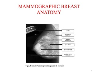
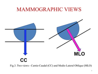
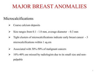
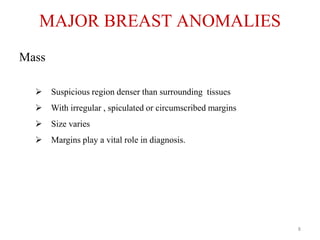
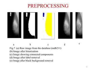
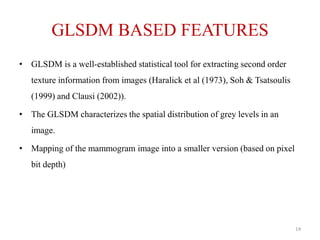
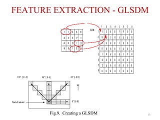
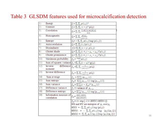
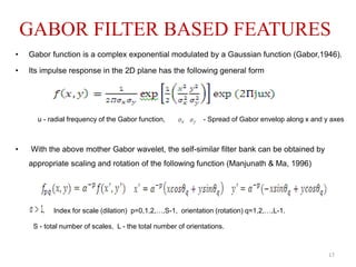
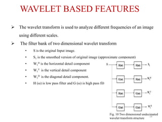
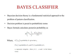
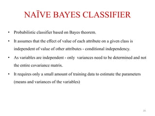
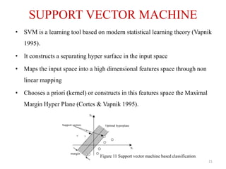
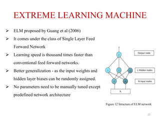
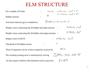
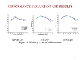
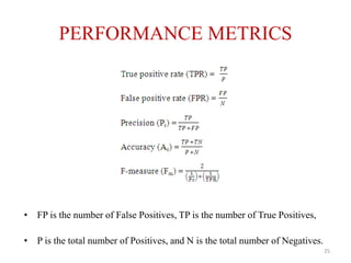
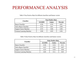
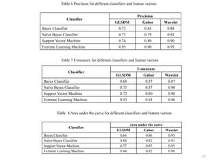
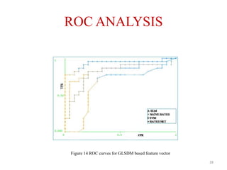
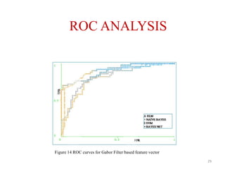
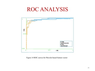
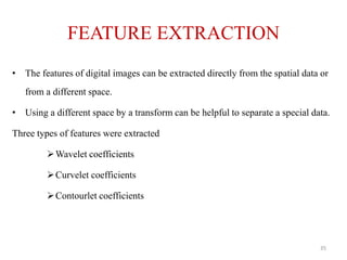
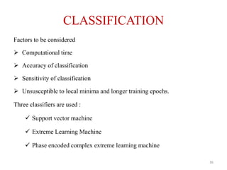
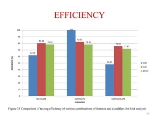
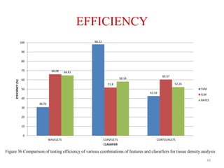
This document proposes a CAD system for analyzing mammogram images to detect breast cancer. It discusses: 1) The need for mammogram analysis and microcalcification/mass detection due to the prevalence of breast cancer. 2) The CAD system which uses preprocessing, feature extraction including GLSDM, Gabor and wavelet transforms, and classifiers like ELM, SVM and Bayes for microcalcification detection, achieving up to 98% accuracy. 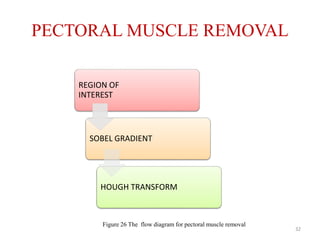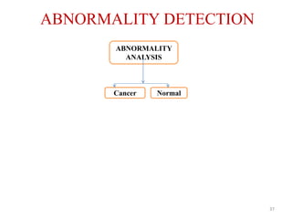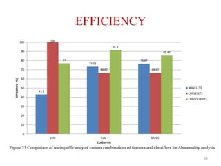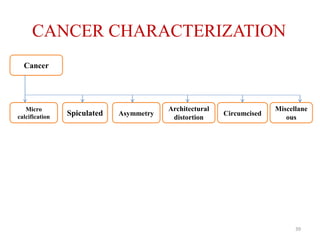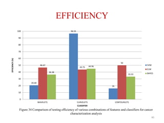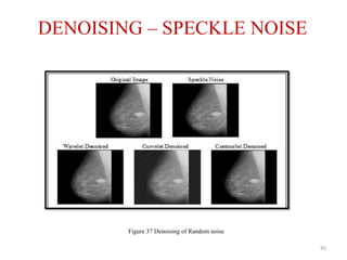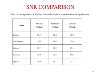3) A comprehensive GUI tool is developed for abnormality detection, cancer characterization, risk analysis and tissue density classification achieving up to 100% accuracy for some classifiers and features. The tool also performs speckle noise denoising.

1. 1
MAMMOGRAM IMAGE ANALYSIS
E.MALAR
Associate Professor & Head
PSG Institute of Technology and Applied Research
Coimbatore

2. OVERVIEW
 Breast Cancer Research Need & Present State – Social Responsibility
 Significance of Mammography
 Need for Preprocessing & Methods
 CAD & Diagnosis
I. Microcalcification Detection
II. Mass & Microcalcification Detection
III.A GUI based Comprehensive tool for Breast Cancer Analysis
2

3. SOCIAL RESPONSIBILITY
 Breast Cancer - Most common cancer among women
 Every year more than 500,000 women die of breast cancer
 Globally, on an average one out of eight women and in India one in 22
women is predicted to develop the disease
 Therapeutic actions are successful in early stage
 Some of the breast lesions are missed during screening by radiologist
3

4. SIGNIFICANCE OF MAMMOGRAPHY
 Identify structural or morphological differences that indicate presence of
cancer
 Conventionally, the image recorded on film and later digital format
 Currently it is the only medical imaging modality used in screening.
 With about 70% sensitivity and 30% positive predictive value,
Mammography screening reduce breast cancer mortality by 25% to 30%
for women in the age group of 50 to 70.
4

5. MAMMOGRAPHIC BREAST
ANATOMY
BREAST
BOUNDARY
DENSE TISSUE
FAT TISSUE
PECTORAL
MUSCLE
LABEL
BLACK BACK
GROUND
Fig.2. Normal Mammogram image and its contents
5

6. MAMMOGRAPHIC VIEWS
CC
MLO
Fig.3. Two views - Carnio Caudal (CC) and Medio Lateral Oblique (MLO)
6

7. MAJOR BREAST ANOMALIES
Microcalcifications
 Coarse calcium deposits
 Size ranges from 0.1 - 1.0 mm, average diameter - 0.3 mm
 Tight clusters of microcalcifications indicate early breast cancer - 3
microcalcifications within 1 sq.cm
 Associated with 30%-50% of malignant cancers
 10%-40% are missed by radiologists due to its small size and non-
palpable
7

8. Mass
 Suspicious region denser than surrounding tissues
 With irregular , spiculated or circumscribed margins
 Size varies
 Margins play a vital role in diagnosis.
MAJOR BREAST ANOMALIES
8

9. I. CAD SYSTEM FOR
MICROCALCIFICATION
DETECTION
9

10. Table 1.MINI –MIAS Database
S.NO. LESION TOTAL
1. Normal 207
2. Spiculated Mass 19
3. Circumscribed Mass 24
4. Microcalcification 25
5. Breast Asymmetry 15
6. Architectural distortion 19
7. Ill-defined mass 15
8. Total 322
10

11. Lesion Risk
No. of images in
Mini-MIAS
No. of Images
used in the
proposed CAD
system
Images used in the proposed CAD system
Normal - 207 30
Dense Glandular - mdb 003, 004, 033, 036,
040, 054, 062, 254, 261, 286.
Fatty - mdb006, 009, 011, 027, 076, 098, 135,
272, 300, 311.
Fatty Glandular – mdb 007, 008, 014, 022,
043, 071, 086, 210, 263, 292.
Microcalcifications
Benign 13 13
mdb 218, 219, 222, 223(2), 226(3), 227, 236,
240, 248, 252.
Malignant 12 12
mdb 209, 211, 213, 231, 238, 239(2), 241,
249(2), 253,256.
Table 2.MINI - MIAS images used in proposed
Microcalcification detection
11

12. Fig.7 .(a) Raw image from the database (mdb211)
(b) Image after binarization
(c) Image showing connected components
(d) Image after label removal
(e) Image after black background removal
PREPROCESSING
12

13.  Gray Level Spatial Dependence Matrix features
(GLSDM)
 Gabor filter based features
 Wavelet Transform based features
FEATURE EXTRACTION
13

14. GLSDM BASED FEATURES
• GLSDM is a well-established statistical tool for extracting second order
texture information from images (Haralick et al (1973), Soh & Tsatsoulis
(1999) and Clausi (2002)).
• The GLSDM characterizes the spatial distribution of grey levels in an
image.
• Mapping of the mammogram image into a smaller version (based on pixel
bit depth)
14

15. FEATURE EXTRACTION - GLSDM
Fig.9. Creating a GLSDM 15

16. Table 3 GLSDM features used for microcalcification detection
16

17. GABOR FILTER BASED FEATURES
• Gabor function is a complex exponential modulated by a Gaussian function (Gabor,1946).
• Its impulse response in the 2D plane has the following general form
u - radial frequency of the Gabor function, - Spread of Gabor envelop along x and y axes
• With the above mother Gabor wavelet, the self-similar filter bank can be obtained by
appropriate scaling and rotation of the following function (Manjunath & Ma, 1996)
Index for scale (dilation) p=0,1,2,…,S-1, orientation (rotation) q=1,2,…,L-1.
S - total number of scales, L - the total number of orientations.
17

18. WAVELET BASED FEATURES
 The wavelet transform is used to analyze different frequencies of an image
using different scales.
 The filter bank of two dimensional wavelet transform
• S is the original Input image.
• S1 is the smoothed version of original image (approximate component)
• W1
H is the horizontal detail component
• W1
V is the vertical detail component
• W1
D is the diagonal detail component.
• H (ω) is low pass filter and G (ω) is high pass filter.
Fig. 10 Two dimensional undecimated
wavelet transform structure
18

19. BAYES CLASSIFIER
• Bayesian decision theory is a fundamental statistical approach to the
problem of pattern classification.
• Decision problem is posed in probabilistic terms
• Bayes formula calculates posterior probability as
Where,
19

20. NAÏVE BAYES CLASSIFIER
• Probabilistic classifier based on Bayes theorem.
• It assumes that the effect of value of each attribute on a given class is
independent of value of other attributes - conditional independency.
• As variables are independent - only variances need to be determined and not
the entire covariance matrix.
• It requires only a small amount of training data to estimate the parameters
(means and variances of the variables)
20

21. SUPPORT VECTOR MACHINE
• SVM is a learning tool based on modern statistical learning theory (Vapnik
1995).
• It constructs a separating hyper surface in the input space
• Maps the input space into a high dimensional features space through non
linear mapping
• Chooses a priori (kernel) or constructs in this features space the Maximal
Margin Hyper Plane (Cortes & Vapnik 1995).
Figure 11 Support vector machine based classification
21

22. EXTREME LEARNING MACHINE
 ELM proposed by Guang et al (2006)
 It comes under the class of Single Layer Feed
Forward Network
 Learning speed is thousand times faster than
conventional feed forward networks.
 Better generalization - as the input weights and
hidden layer biases can be randomly assigned.
 No parameters need to be manually tuned except
predefined network architecture
Figure 12 Structure of ELM network
22

23. ELM STRUCTURE
For a sample of N data -
Hidden neurons -
Activation function g(x) is modeled as
Weight vector connecting the ith hidden and input neurons -
Weight vector connecting the ith hidden and output neurons -
Output vector of SLFN -
Threshold of ith hidden neuron -
These N equations can be written compactly as given by
The resulting training error is minimized by solving
Its least square solution with minimum norm is given by
23

24. (a) GLSDM (b) Gabor (c) Wavelet
Figure 13 Efficiency vs. No. of hidden neurons
PERFORMANCE EVALUATION AND RESULTS
0 10 20 30 40 50 60 70 80 90
0
10
20
30
40
50
60
70
80
90
100
Efficiency(%)
Number of Hidden Neurons
Unipolar
Gaussian
Bipolar
0 10 20 30 40 50 60 70 80
0
10
20
30
40
50
60
70
80
90
Efficiency(%)
Number of Hidden Neurons
Unipolar
Gaussian
Bipolar
0 10 20 30 40 50 60 70 80
0
10
20
30
40
50
60
70
80
90
100
Efficiency(%)
Number of Hidden Neurons
Unipolar
Gaussian
Bipolar
24

25. PERFORMANCE METRICS
• FP is the number of False Positives, TP is the number of True Positives,
• P is the total number of Positives, and N is the total number of Negatives.
25

26. PERFORMANCE ANALYSIS
Classifier
True Positive Rate
GLSDM Gabor Wavelet
Bayes Classifier 0.70 0.74 0.87
Naïve Bayes Classifier 0.72 0.61 0.90
Support Vector Machine 0.72 0.80 0.90
Extreme Learning Machine 0.90 0.95 0.98
Classifier
False Positive Rate
GLSDM Gabor Wavelet
Bayes Classifier 0.30 0.18 0.11
Naïve Bayes Classifier 0.27 0.28 0.07
Support Vector Machine 0.25 0.20 0.09
Extreme Learning Machine 0.05 0.11 0.05
Table 4 True Positive Rate for different classifiers and feature vectors
Table 5 False Positive Rate for different classifiers and feature vectors
26

27. Classifier
Area under the curve
GLSDM Gabor Wavelet
Bayes Classifier 0.66 0.86 0.95
Naïve Bayes Classifier 0.84 0.82 0.93
Support Vector Machine 0.77 0.87 0.95
Extreme Learning Machine 0.94 0.92 0.98
Classifier
Precision
GLSDM Gabor Wavelet
Bayes Classifier 0.73 0.84 0.88
Naïve Bayes Classifier 0.75 0.79 0.92
Support Vector Machine 0.74 0.80 0.90
Extreme Learning Machine 0.95 0.90 0.95
Classifier
F-measure
GLSDM Gabor Wavelet
Bayes Classifier 0.68 0.37 0.87
Naïve Bayes Classifier 0.75 0.57 0.90
Support Vector Machine 0.72 0.80 0.90
Extreme Learning Machine 0.93 0.93 0.96
Table 6 Precision for different classifiers and feature vectors
Table 7 F-measure for different classifiers and feature vectors
Table 8 Area under the curve for different classifiers and feature vectors
27

28. ROC ANALYSIS
Figure 14 ROC curves for GLSDM based feature vector
28

29. Figure 14 ROC curves for Gabor Filter based feature vector
ROC ANALYSIS
29

30. Figure 14 ROC curves for Wavelet based feature vector
ROC ANALYSIS
30

31. III. A GUI BASED COMPREHENSIVE
TOOL FOR BREAST CANCER
ANALYSIS
31

32. PECTORAL MUSCLE REMOVAL
REGION OF
INTEREST
SOBEL GRADIENT
HOUGH TRANSFORM
32
Figure 26 The flow diagram for pectoral muscle removal

33. REGION OF INTEREST
• Pectoral muscle would
be present in the top
half of the image.
33Figure 27 The ROI selection for pectoral line detection

34. SOBEL GRADIENT
ROI
34Figure 28 (a) ROI and (b) output of Sobel gradient

35. FEATURE EXTRACTION
• The features of digital images can be extracted directly from the spatial data or
from a different space.
• Using a different space by a transform can be helpful to separate a special data.
Three types of features were extracted
Wavelet coefficients
Curvelet coefficients
Contourlet coefficients
35

36. CLASSIFICATION
Factors to be considered
 Computational time
 Accuracy of classification
 Sensitivity of classification
 Unsusceptible to local minima and longer training epochs.
Three classifiers are used :
 Support vector machine
 Extreme Learning Machine
 Phase encoded complex extreme learning machine
36

37. ABNORMALITY
ANALYSIS
Cancer Normal
ABNORMALITY DETECTION
37

38. EFFICIENCY
43.1
73.33
76.67
100
66.67 66.67
77
91.3
85.47
0
10
20
30
40
50
60
70
80
90
100
SVM ELM BAYES
EFFICIENCY(%)
CLASSIFIER
WAVELETS
CURVELETS
CONTOURLETS
38
Figure 33 Comparison of testing efficiency of various combinations of features and classifiers for Abnormality analysis

39. CANCER CHARACTERIZATION
Cancer
Micro
calcification Spiculated Asymmetry
Architectural
distortion
Circumcised
Miscellane
ous
39

40. EFFICIENCY
20.68
96.55
16
46.67
43.75
50
36.38
44.96
33.33
0
10
20
30
40
50
60
70
80
90
100
WAVELETS CURVELETS CONTOURLETS
EFFICIENCY(%)
CLASSIFIER
SVM
ELM
BAYES
40
Figure 34 Comparison of testing efficiency of various combinations of features and classifiers for cancer
characterization analysis

41. RISK ANALYSIS
RISK ANALYSIS
Benign Malignant
41

42. EFFICIENCY
62.06
100
48.27
80.31
82.31
75.86
78.39 78.36
71.87
0
10
20
30
40
50
60
70
80
90
100
WAVELETS CURVELETS CONTOURLETS
EFFICIENCY(%)
CLASSIFIER
SVM
ELM
BAYES
42
Figure 35 Comparison of testing efficiency of various combinations of features and classifiers for Risk analysis

43. TISSUE DENSITY ANALYSIS
TISSUE DENSITY
Fatty
Fatty
glandular
Dense
glandular
43

44. EFFICIENCY
30.76
98.22
42.59
66.08
51.8
60.37
64.81
58.14
52.24
0
10
20
30
40
50
60
70
80
90
100
WAVELETS CURVELETS CONTOURLETS
EFFICIENCY(%)
CLASSIFIER
SVM
ELM
BAYES
44
Figure 36 Comparison of testing efficiency of various combinations of features and classifiers for tissue density analysis

45. DENOISING – SPECKLE NOISE
45
Figure 37 Denoising of Random noise

46. SNR COMPARISON
Noises
Wavelet
SNR/dB
Contourlet
SNR/dB
Curvelet
SNR/dB
Random 21.59 23.65 16.51
Salt & pepper 6.76 11.65 32.94
Poisson 25.71 25.55 23.14
Gaussian 16.96 17.84 57.51
Speckle 16.69 19.13 22.13
46
Table 16 Comparison Of Wavelet, Contourlet And Curvelet Based Denoising Methods

47. SCOPE FOR FUTURE WORK
 The clinical information may be added to help in epidemiological studies.
 Mammograms can be combined with different imaging modalities like
MRI and Ultrasound.
 Dense breast tissue difficult in classifying begin and malignant breast
disease.
 Categorize the different types of mass.

48. THANK YOU
48