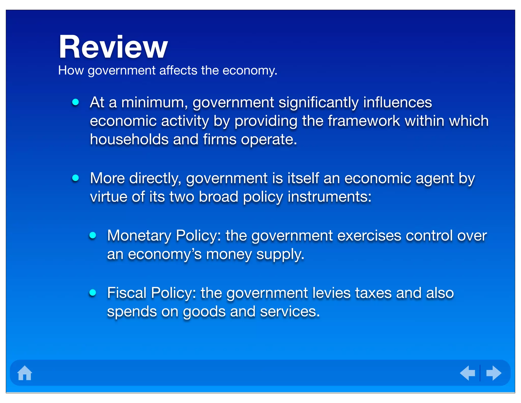
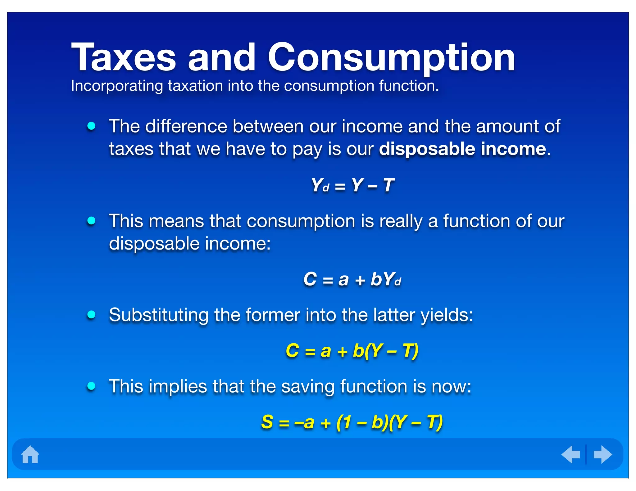
The document analyzes the role of government in the economy, focusing on fiscal policy, which entails taxation and government spending. It outlines how taxes influence disposable income and consumption, and how government spending impacts equilibrium output. Lastly, it discusses the effects of fiscal stimuli during economic downturns and overheating, and examines balanced budget spending.

1. GOVernment in the economy
Part I: The Effects of Fiscal Policy

2. Review
• At a minimum, government significantly influences
economic activity by providing the framework within which
households and firms operate.
• More directly, government is itself an economic agent by
virtue of its two broad policy instruments:
• Monetary Policy: the government exercises control over
an economy’s money supply.
• Fiscal Policy: the government levies taxes and also
spends on goods and services.
How government affects the economy.

3. Taxation
• Taxes represent funds that have to be paid to the
government out of our income.
• This means that our incomes have to be divided not just
between savings and consumption, but taxes as well:
Y = C + S + T
• The taxes that government collects (T) are what finance
government expenditure (G).
• If G < T, the government is running a surplus.
• If G > T, the government is running a deficit.
• If G = T, we have a balanced budget.
Some insights into how taxes factor into economic analysis.

4. Taxes and Consumption
• The difference between our income and the amount of
taxes that we have to pay is our disposable income.
Yd = Y – T
• This means that consumption is really a function of our
disposable income:
C = a + bYd
• Substituting the former into the latter yields:
C = a + b(Y – T)
• This implies that the saving function is now:
S = –a + (1 – b)(Y – T)
Incorporating taxation into the consumption function.

5. Government Spending
• Consider: whether government spends or not does not
necessarily have anything to do with how the economy is
doing.
• Government projects can be undertaken for political
rather than economic reasons.
• Government can (hypothetically) spend whether or not it
has the necessary funds to finance its projects.
• If this is the case, we can consider government spending
as another autonomous variable.
Putting the “G” in Planned Aggregate Expenditure (i.e. C + I + G).

6. Output and Fiscal Policy
• A more complete model of planned aggregate expenditure:
AE = C + I + G
• Substituting:
AE = a + b (Y – T) + I + G
• The equilibrium condition:
Y = AE
• Thus (and rearranging):
Y = (a + I + G) + bY – bT
Putting it all together.

7. Output and Fiscal Policy
Putting it all together.
We have now derived the equilbrium condition:
Y = 1 ( a + I + G – bT)
1 – b
Consider:
Any change in government
spending changes equilibrium
output by:
Any change in taxation
changes equilibrium output by:
1 – b
1
1 – b
b
–

8. Output and Fiscal Policy
Putting it all together.
We have now derived the equilbrium condition:
Y = 1 ( a + I + G – bT)
1 – b
Consider:
Any change in government
spending changes equilibrium
output by:
Any change in taxation
changes equilibrium output by:
MPS
1
MPS
MPC
–

9. Output and Fiscal Policy
Putting it all together.
We have now derived the equilbrium condition:
Y = 1 ( a + I + G – bT)
1 – b
The Government
Spending Multiplier:
The Tax Multiplier:
MPS
1
MPS
MPC
–

10. Fiscal Stimuli
• Recessions represent a downturn in economic performance.
• Recall: they are defined as a decline in output over two
consecutive quarters.
• If ouput declines, it must mean that investments have
declined.
• Government spending can be an effective tool to offset
recessions.
Case 1: Recession
1
MPS
– ∆ I
1
MPS
∆ G
Decrease in Planned
Investments
Increase in Government
Spending
+ = 0

11. Fiscal Stimuli
• An economy may be said to be “overheating” when
economic performance leads to rapidly rising output and
income over a short interval.
• The immediate consequence of this is rising inflation and a
rising cost of living.
• Overheating is often kept in check by a commensurate
increase in taxes.
• Fiscal Drag: with rising incomes come rising tax revenue.
Case 2: “Overheating”

12. Fiscal Stimuli
Case 3: Balanced Budget Spending
∆ G = ∆ T
What would happen if the govenrment finances an
increase in expenditure by an equal increase in taxes?
From the multiplier:
The change in equilibrium output from a
change in taxes is given by:
MPS
MPC
– ∆ T
The change in equilibrium output from a
change in government spending is given by: MPS
1
∆ G

13. Fiscal Stimuli
Case 3: Balanced Budget Spending
The total change in output from “balanced budget spending”:
∆ Y =
MPS
MPC
– ∆ T
MPS
1
∆ G
Since ∆ G = ∆ T:
∆ Y =
MPS
MPC
– ∆ G
MPS
1
∆ G

14. Fiscal Stimuli
Case 3: Balanced Budget Spending
Simplifying:
∆ Y =
MPS
1 - MPC
∆ G
However, (1 – MPC) = MPS! Therefore:
∆ Y =
MPS
MPS
∆ G
∆ Y = ∆G