Downloaded 18 times
![Simplifications
• Recall that all variables are aggregates.
• Since people only care about the “real” value of their
income/output, we can assume that all variables under
consideration are expressed in real terms.
• To proceed with the analysis, we can consider the simplest
case:
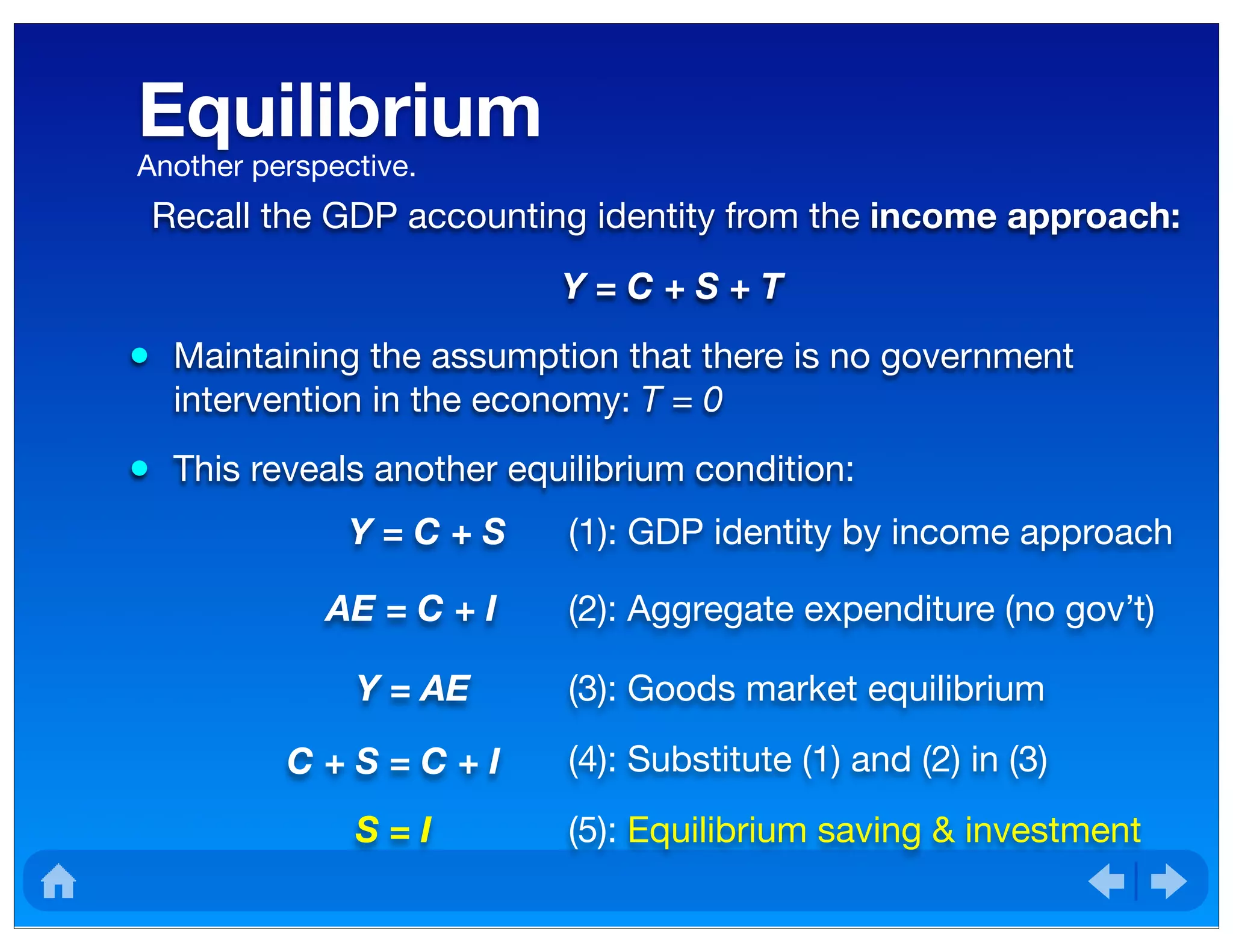
• There is no government intervention in the economy
(i.e. G = 0).
• A closed economy model (i.e. [X – M] = 0).
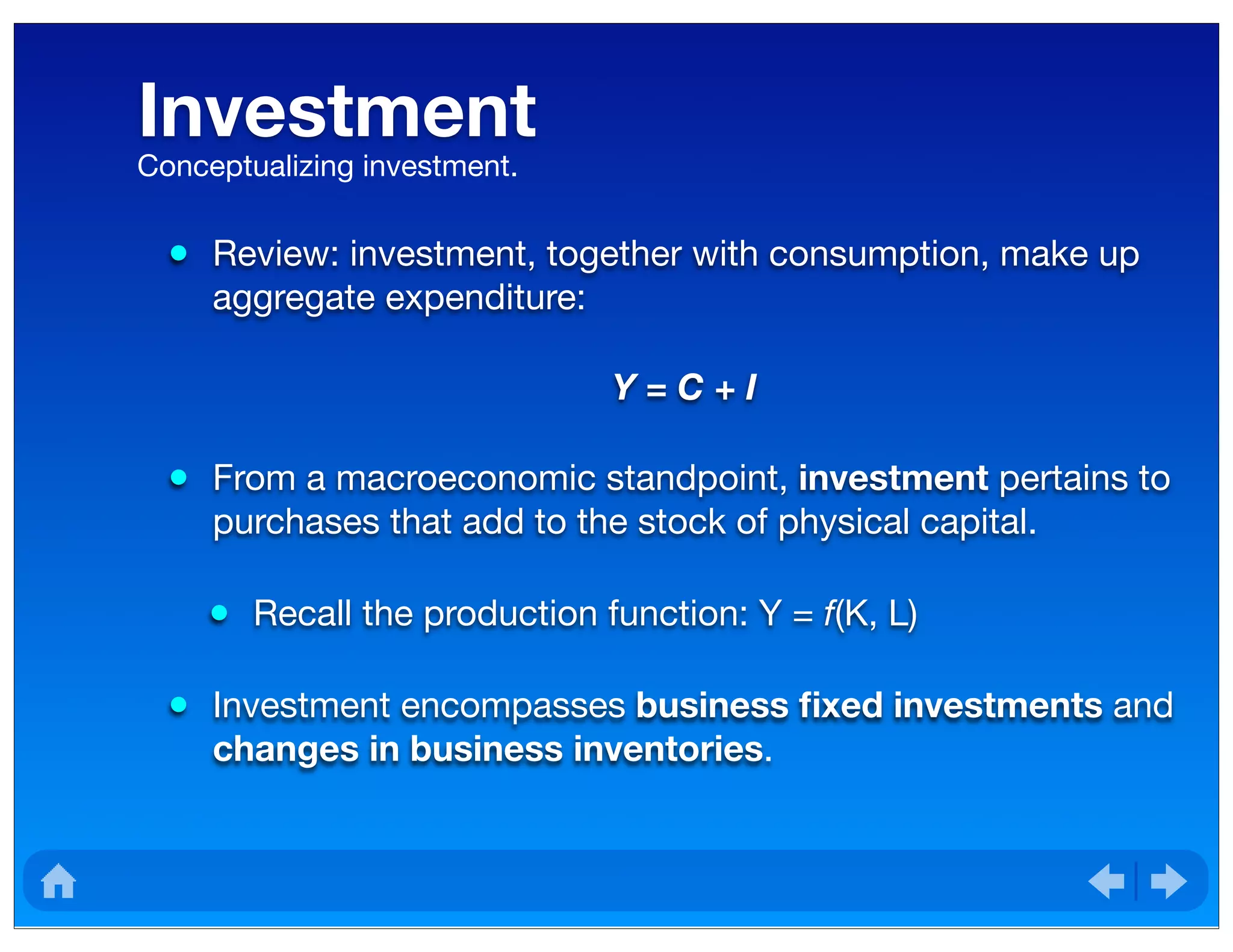
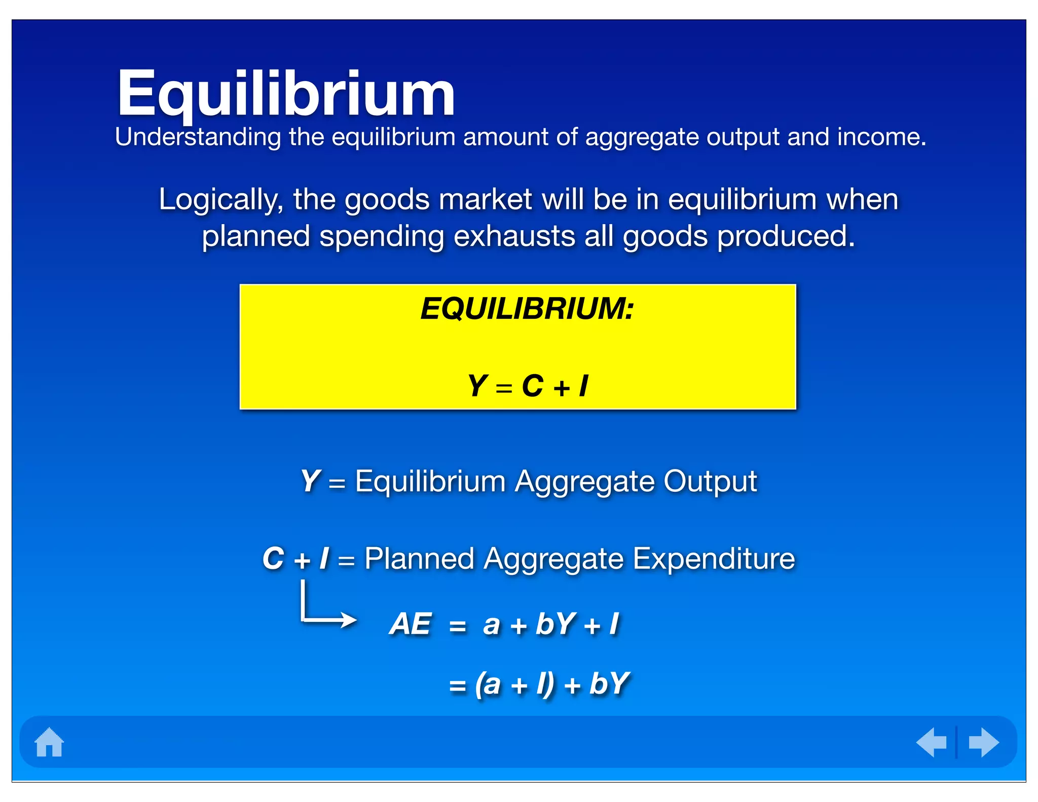
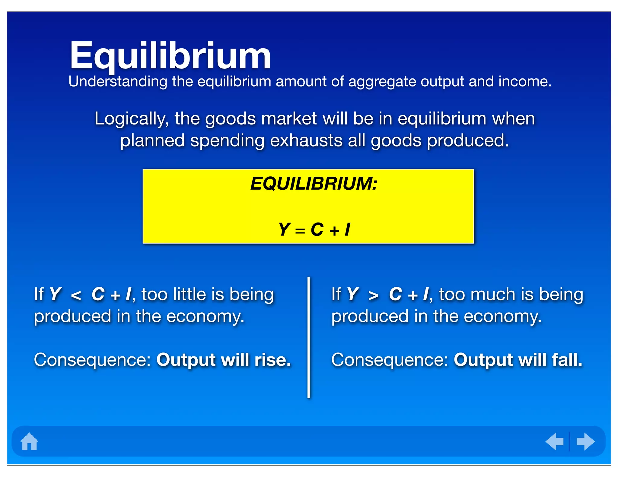
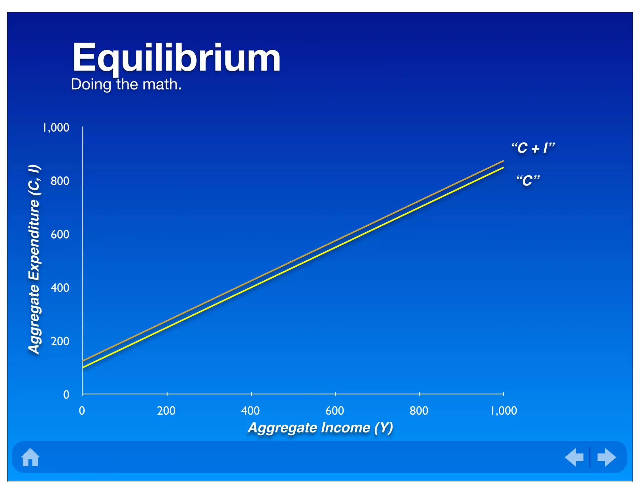
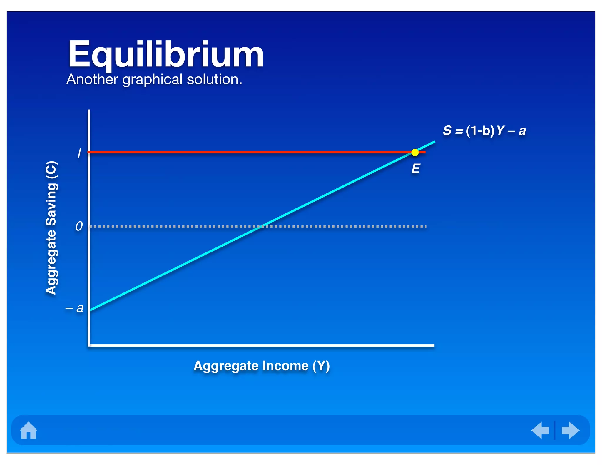
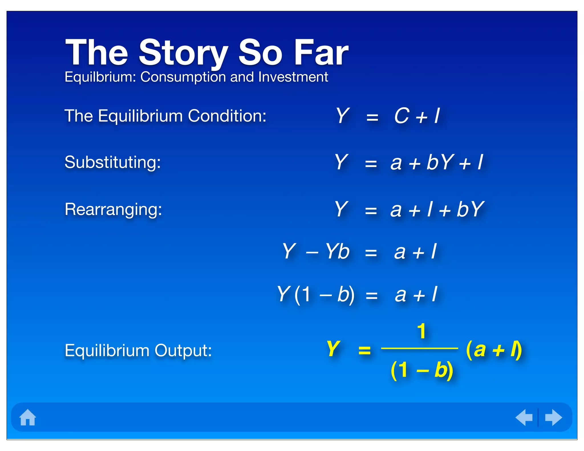
• Thus, our model reduces to:
Y = C + I
Some assumptions to make the analysis easier.](https://image.slidesharecdn.com/lecture9consumptiontheory-151216145957/75/Macroeconomic-Consumer-Theory-3-2048.jpg)
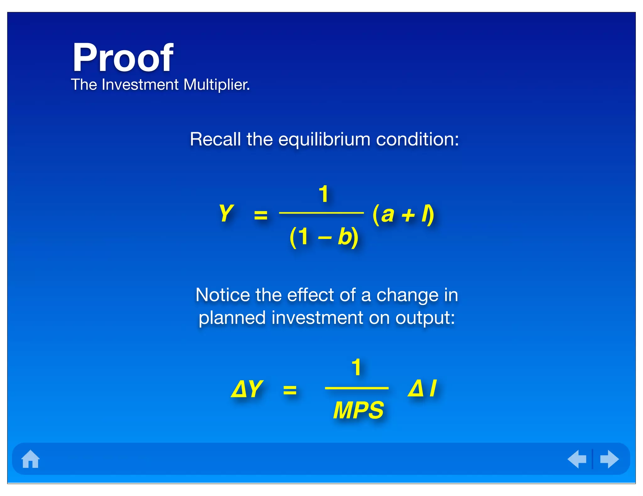
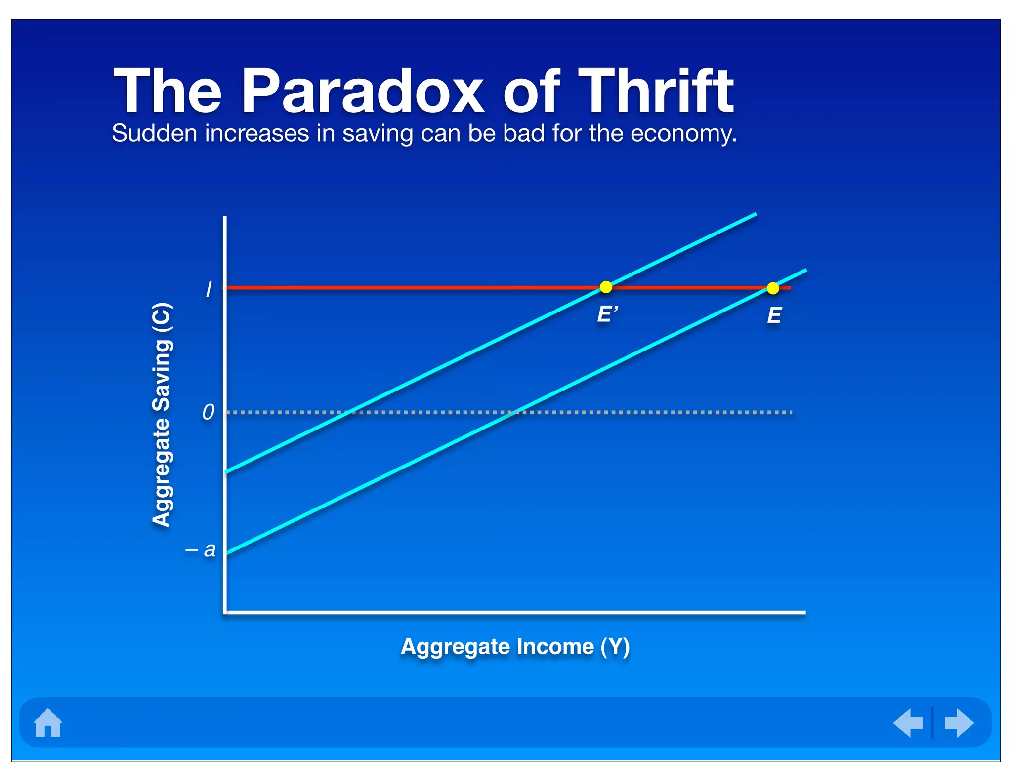

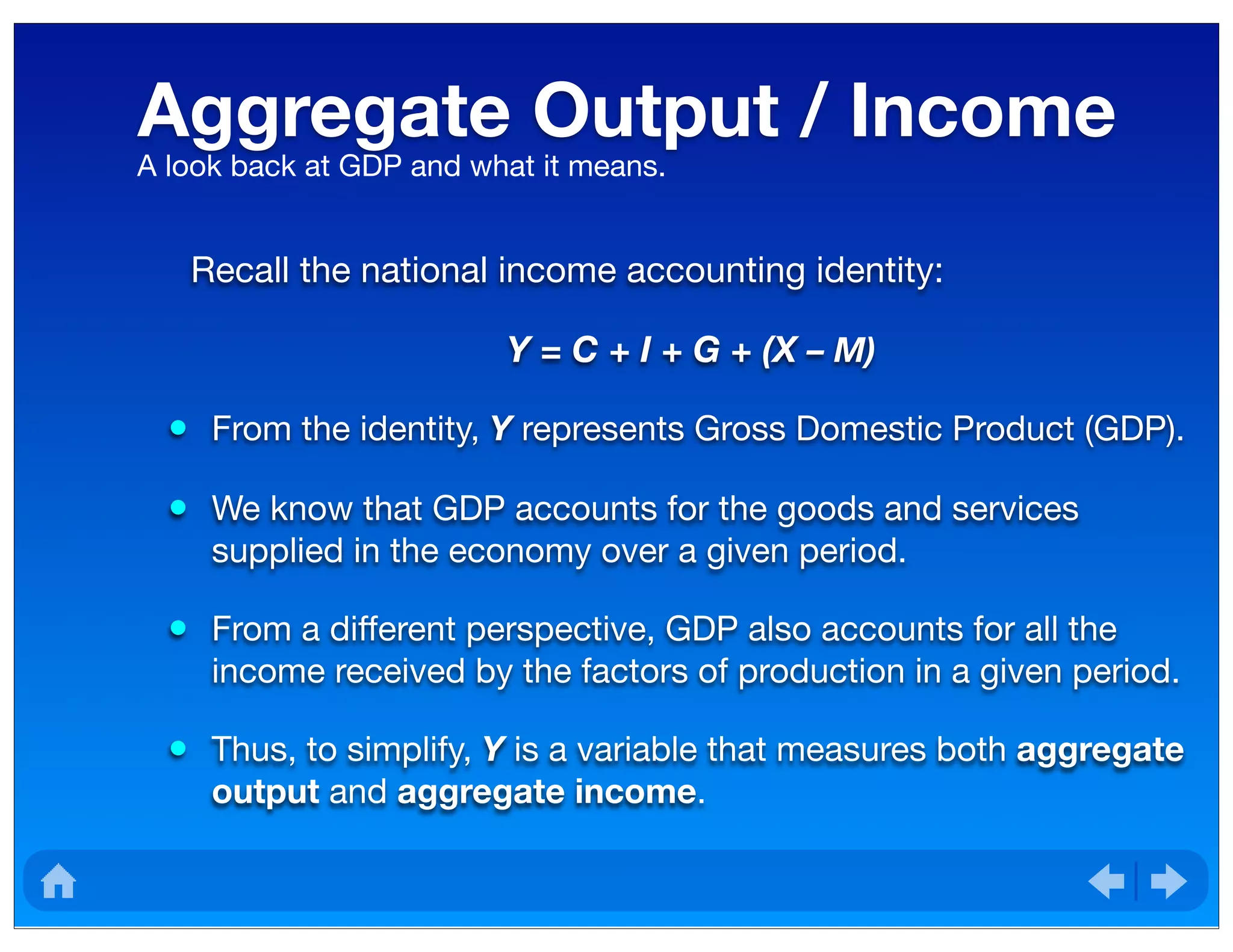
The document explains the national income accounting identity, emphasizing that Gross Domestic Product (GDP) represents both aggregate output and income. It discusses consumption and saving behavior based on the Keynesian consumption and saving functions, as well as the impact of investment on the economy. Furthermore, it examines equilibrium conditions in the goods market and the effects of changes in consumption and investment on overall output.


![Gross Domestic Product [What is not included]](https://cdn.slidesharecdn.com/ss_thumbnails/gross-domestic-product-what-is-not-included-12300-thumbnail.jpg?width=640&height=640&fit=bounds)