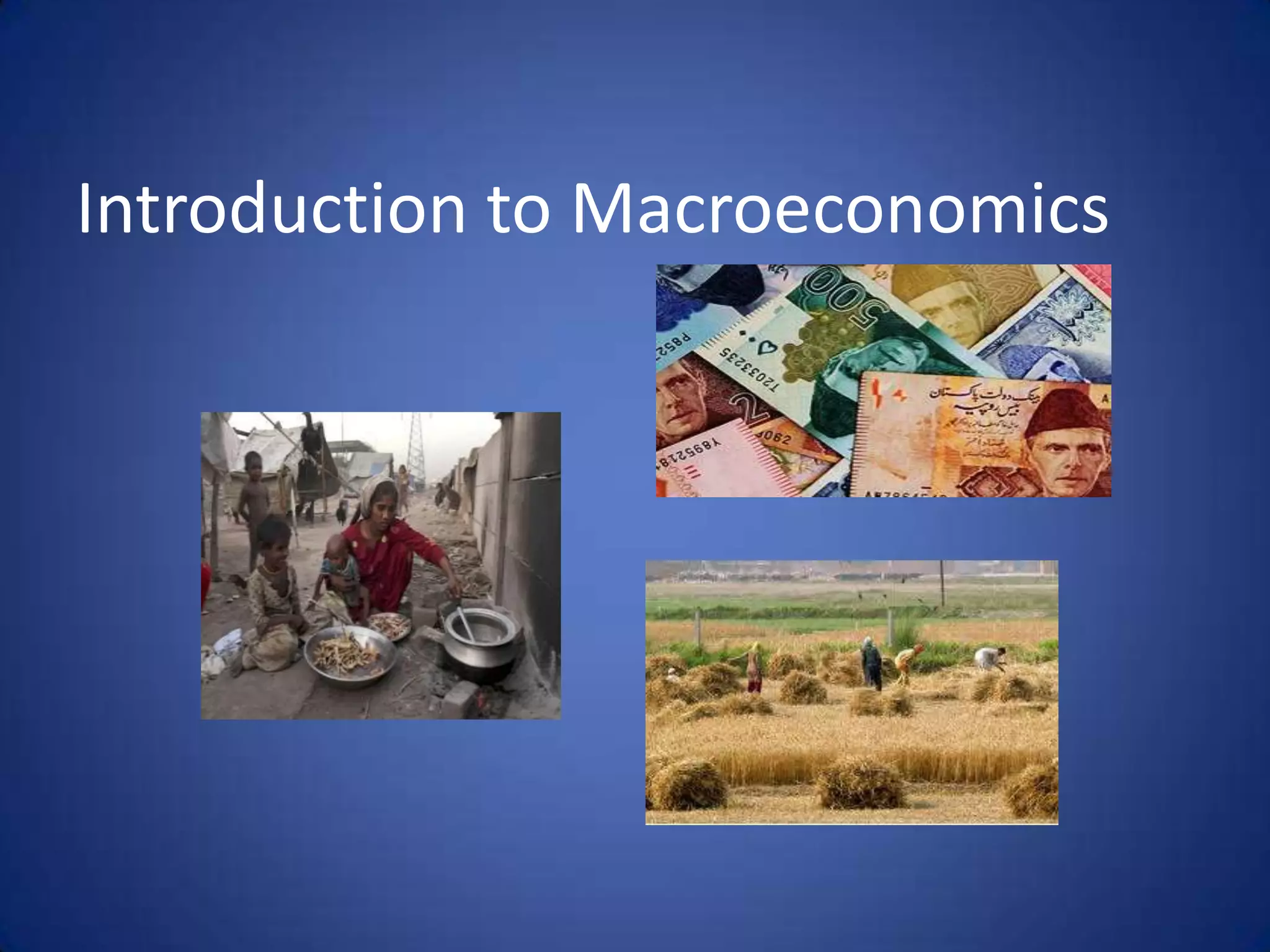
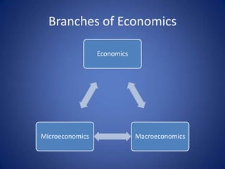
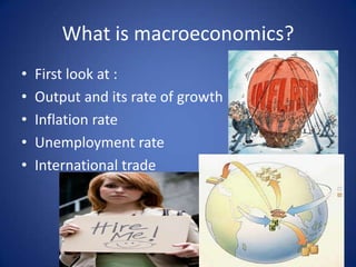
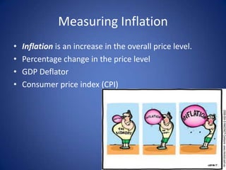
This document provides an introduction to macroeconomics. It discusses that macroeconomics examines the economy as a whole by looking at aggregates like income, consumption, investment, and prices. It then covers key macroeconomic concepts like measuring GDP, inflation, unemployment, and international trade. It introduces three models used in macroeconomics: the long-run model of economic growth, the aggregate supply and aggregate demand model for the short-run and medium-run, and the business cycle model.

1. Introduction to Macroeconomics

2. Branches of Economics
Economics
Microeconomics Macroeconomics

3. Branches of Economics
• Microeconomics examines the behavior of
individual decision-making units—business
firms and households.

4. • Macroeconomics deals with the economy as a whole; it
examines the behavior of economic aggregates such as
aggregate income, consumption, investment, and the overall
level of prices.
– Aggregate behavior refers to the behavior of all households and
firms together.

5. What is macroeconomics?
• First look at :
• Output and its rate of growth
• Inflation rate
• Unemployment rate
• International trade

6. Measuring Economic growth
• Gross Domestic Product (GDP)
Value of all the final goods and services produced
within a country in given period of time.
• Real GDP
The volume of goods and services produced within a
country (i.e. GDP adjusted for inflation)
• Economic growth
Percentage rate of increase of real GDP

7. Measuring Inflation
• Inflation is an increase in the overall price level.
• Percentage change in the price level
• GDP Deflator
• Consumer price index (CPI)

8. Measuring Unemployment
• Labor force = employed + unemployed
• Unemployment rate = unemployment/labor force
• Unemployment= Does not have a job and has been
seeking for a job for past 4 weeks.
• The long term unemployment is the share of
unemployed persons since
12 months and more in the
total numbers of the active
persons in labor market.

9. International trade/ Trade balance
• The balance between imports and exports.
• Balance of trade = exports are equal to
imports.

10. Three Models
• Macroeconomics is organised around three
models
• Each model is concerned with different time
frames
– The long run
– The medium run
– The short run
• Let’s consider each in more detail

11. Very Long Run Economic Growth
• Growth theory describes the long run
behaviour of the economy
• The time is usually measured in multiples of
decades (e.g. 20 years or more)
• The focus is on the average growth in
important macroeconomic variables
• Short-run fluctuations in important variables
like employment, investment and output are
ignored

12. Very Long Run Economic Growth
• The long run level of output is determined
solely by supply-side considerations
• That is, output is determined by the
productive capacity of the economy
• All factors of production are assumed to be
fully employed
• Economic growth is, therefore, a function of
increases in productive capacity

13. Very Long Run Economic Growth
• Differences in average growth rates of
economies are important
• Major causes of economic growth are
– Development of new technology
– Accumulation of physical and human capital
– Appropriate provision of infrastructure
– Higher rates of domestic saving

14. Very Long Run Economic Growth
• Economic growth determines the changes in the
standard of living
• A country growing at an average of 4% per year
instead of 2% will have a 50% higher standard of
living over a generation of 20 years
• This higher 4% average annual growth rate will
lead to a seven fold increase in the standard of
living over 100 years!
• Let’s now introduce a model which will be useful
for our analysis

15. Fixed Productive Capacity
• What determines the change in the overall
price level (the inflation rate)?
• The aggregate supply (AS)–aggregate
demand (AD) model explains short- to
medium-run determination of inflation and
real output
• In the long run the productive capacity of the
economy is assumed to be constant

16. Fixed Productive Capacity
• This is represented by a vertical AS schedule
at real output level Y0
P AS
Price Level
Y0 Y

17. Fixed Productive Capacity
• The AD schedule represents, for each price
level, the level of output where both the
goods and money markets are in equilibrium
• These schedules will be fully explained in
next lectures
• The intersection of the AS and AD schedules
determines the price (P0) and real output (Y0)

18. Fixed Productive Capacity
• AD and AS in the long run
What happens when AD
P AS shifts rightwards?
AD
Price increases
Price Level
P0 What happens when AS shifts
rightwards?
Price decreases
Y0 Y

19. The Short Run
• Short-run fluctuations in real output are
important
• AD is the major determinant of these
variations
• In the short run the price level is pegged at
P0 making the short-run AS schedule
horizontal

20. The Short Run
• AD and AS in the short run
What happens when AD
P shifts rightwards?
Price unchanged
Price Level
P0 AS
AD
Y0 Y

21. The Medium Run
• How do we describe the transition between
the short run and long run?
• High AD pushes real output above Y0
(according to the long-run model)
• Over time, firms will increase prices and the
AS curve will move upwards
• The medium run will give an upsloping AS
curve

22. The Medium Run
• The relative steepness of the AS curve is a
major controversy in macroeconomics
P
Price Level
P0
AS AD
Y0 Y

23. To Reiterate …
• Growth theory, AS and AD form a very
important framework for the further
analysis of
– Growth and GDP
– The business cycle
• Let’s consider each in turn

24. Growth and GDP

25. The Business Cycle and GDP
• The business cycle describes the variation of
economic activity around the path of trend
growth
• Inflation, growth and unemployment all
demonstrate cyclical patterns
• The output gap measures the difference
between actual and potential output:
Output gap = potential output – actual output

26. • Potential Output:
Total gross domestic product (GDP) that could be
produced by an economy if all its resources were
fully employed.
• Actual Output
Actual output is the "real" GDP ( gross domestic
product).

27. The Business Cycle and Inflation
• Increases in inflation are inversely related to
the output gap
• Expansionary AD policies tend to produce
inflation when unemployment is relatively
low
• The cost of the cycle above trend is inflation
and the cost below trend is unemployment

28. Business Cycle Features
• Business cycles have common characteristics
• Procyclical variables rise with expansionary
business activity (e.g.
output, employment, interest rates and
money supply)
• Countercyclical variables (like inventories and
bankruptcies) move in the opposite direction
to business activity

29. • Procyclical has a different meaning in the
context of economic policy. In this context, it
refers to any aspect of economic policy that
could magnify economic or financial
fluctuations.
• An economic policy that is believed to
decrease fluctuations is called countercyclical.

30. Business Cycle Features
• Some variables exhibit more variability than
others (e.g. inventories are volatile while
consumption is smooth, especially relative to
output)
• The impulse-propagation model describes:
– how a shock (impulse) disturbs the economy
from a long-run trend
– which lasts (propagates) over time
• Economists disagree over possible
propagation mechanisms

31. Business Cycle Features
• There are three broad types of shocks
– Policy shocks which affect fiscal expenditure
and interest rates (e.g. fiscal and monetary
policies)
– Supply shocks which affect production and
price-setting (e.g. technology advances)
– Private sector shocks which affect aggregate
demand (e.g. changes in private investment)

32. Business Cycle Features
• There is debate about the actual timing of
business cycles
• Which measure should be used?
– Variables like unemployment lag changes in
real GDP (called lagging indicators)
– Leading indicators like firms’ profitability and
building approvals precede changes in GDP
– Aggregating variables into a composite index
will give a coincident index to measure turning
points in the business cycle

33. Business Cycle Features
• Another debate concerns separating the
cycle from trend
– The classical business cycle considers actual
levels so that a fall in GDP describes negative
growth
– Two consecutive quarters of negative growth
in real GDP is called a (classical) recession
– The growth cycle considers fluctuations in
growth rates of the economy around the trend
growth rate

34. 1.3 Schools of Thought
• During the 1960s there were two main
views
– The monetarists believed the economy is best
left to itself
– The Keynesian’s argued that government
intervention could improve economic
performance
• Two schools have developed since then
– the new classical school in the 1970s
– the Keynesian school in the 1980–90s

35. New Classical School
• Consistent with the monetarist view
– Economic agents optimise
– Decisions rationally use all available
information (rational expectations)
– Markets are assumed to clear
• These assumptions ensure there is no
involuntary unemployment
• The real business cycle extension argues that
real supply side shocks are the major causes
of fluctuations in economic activity

36. New Keynesian School
• Extends the earlier Keynesian view that
markets will not always clear even if agents
are maximising
• Reasons are varied and include
– There is incomplete information
– Institutions affect the workings of markets
– Costs of changing wages and prices lead to
price rigidities
• These reasons explain fluctuations in output
and employment

37. Economic Controversies
• The two main competing views of modern
macroeconomics are highlighted in real-
world political and media discussions
• Frequently these differences are exaggerated
in debate
• There are significant areas of agreement
• Debate and research continually evolve new
areas of consensus e.g. there is increasing
agreement on information problems with
wage-price setting

38. Thanks