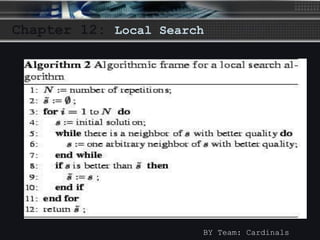
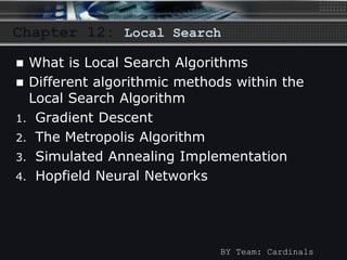
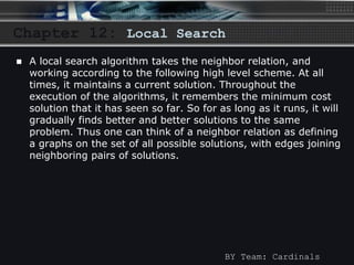
The document discusses local search algorithms, including gradient descent, the Metropolis algorithm, simulated annealing, and Hopfield neural networks. It provides details on how each algorithm works, such as gradient descent taking steps proportional to the negative gradient of a function to find a local minimum. The algorithms are compared, with some having similarities in their methods, like maximum cut problem and Hopfield neural networks using state flipping algorithms, and Metropolis and gradient descent using simulated annealing. Advantages and disadvantages of local search algorithms are presented.

![Chapter 12: Local Search
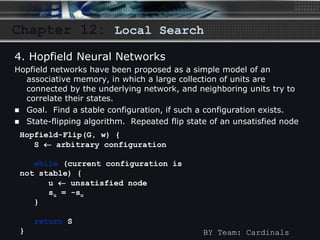
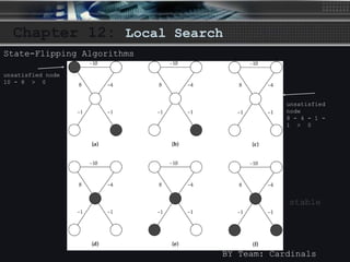
BY Team: Cardinals
2. The Metropolis Algorithm
[Metropolis, Rosenbluth, Rosenbluth, Teller, Teller 1953]
– Step by Step Simulation behavior of a physical
system according to principles of statistical
mechanics.
– Simulation maintains a current state of the
system and tries to produce a new state by
applying a perturbation to this state.](https://image.slidesharecdn.com/localsearchalgorithms-140922035204-phpapp02/85/Local-search-algorithms-9-320.jpg)

![Chapter 12: Local Search
3. Simulated Annealing Implementation
Simulated annealing is a generic probabilistic meta-algorithm for
the global optimization problem, namely locating a good
approximation to the global minimum of a given function in a
large search space.
Simulated annealing is a generalization of a Monte Carlo method for
examining the equations of state and frozen states of n-body
systems [Metropolis et al. 1953]
Simulated annealing has been used in various combinatorial
optimization problems and has been particularly successful in circuit
design problems.
BY Team: Cardinals](https://image.slidesharecdn.com/localsearchalgorithms-140922035204-phpapp02/85/Local-search-algorithms-12-320.jpg)