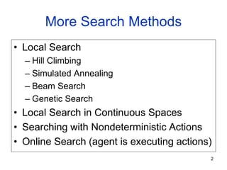
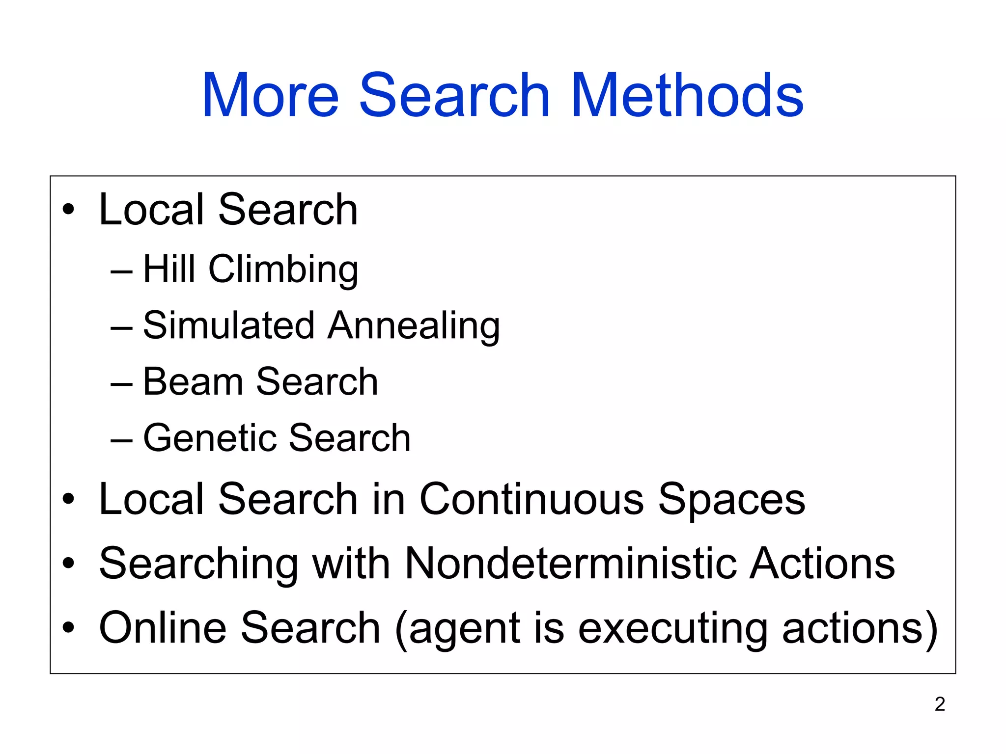
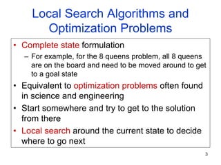
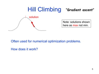
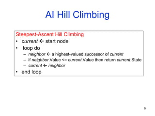
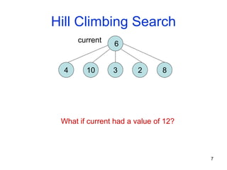
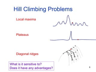
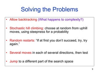
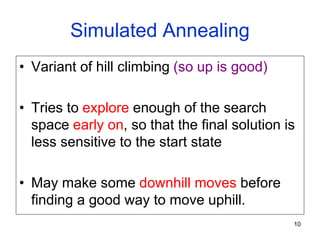
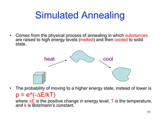
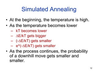
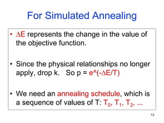
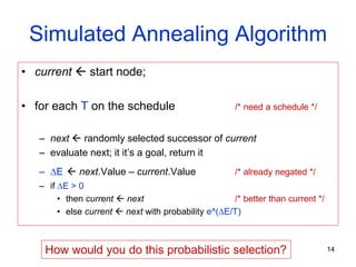
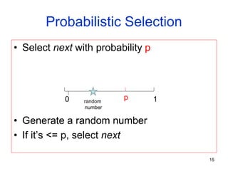
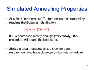
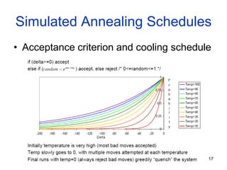
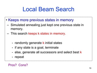
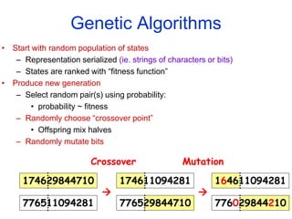
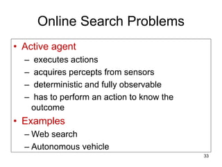
The document discusses various search methods including local search techniques like hill climbing, simulated annealing, beam search, and genetic search. It also covers searching continuous state spaces, nondeterministic actions, and online search where the agent performs actions and acquires sensor data. Local search methods start from an initial state and try to improve the current state to reach the goal. Simulated annealing allows occasional downhill moves to help explore more of the search space.

1. More Search Methods
• Local Search
– Hill Climbing
– Simulated Annealing
– Beam Search
– Genetic Search
• Local Search in Continuous Spaces
• Searching with Nondeterministic Actions
• Online Search (agent is executing actions)
2

2. 3
Local Search Algorithms and
Optimization Problems
• Complete state formulation
– For example, for the 8 queens problem, all 8 queens
are on the board and need to be moved around to get
to a goal state
• Equivalent to optimization problems often found
in science and engineering
• Start somewhere and try to get to the solution
from there
• Local search around the current state to decide
where to go next

3. Pose Estimation Example
• Given a geometric model of a 3D object
and a 2D image of the object.
• Determine the position and orientation of
the object wrt the camera that snapped the
image.
image 3D object
• State (x, y, z, x-angle, y-angle, z-angle) 4

4. 5
Hill Climbing “Gradient ascent”
solution
Note: solutions shown
here as max not min.
Often used for numerical optimization problems.
How does it work?

5. 6
AI Hill Climbing
Steepest-Ascent Hill Climbing
• current  start node
• loop do
– neighbor  a highest-valued successor of current
– if neighbor.Value <= current.Value then return current.State
– current  neighbor
• end loop

6. 7
Hill Climbing Search
6
4 10 3 2 8
current
What if current had a value of 12?

7. 8
Hill Climbing Problems
Local maxima
Plateaus
Diagonal ridges
What is it sensitive to?
Does it have any advantages?

8. 9
Solving the Problems
• Allow backtracking (What happens to complexity?)
• Stochastic hill climbing: choose at random from uphill
moves, using steepness for a probability
• Random restarts: “If at first you don’t succeed, try, try
again.”
• Several moves in each of several directions, then test
• Jump to a different part of the search space

9. 10
Simulated Annealing
• Variant of hill climbing (so up is good)
• Tries to explore enough of the search
space early on, so that the final solution is
less sensitive to the start state
• May make some downhill moves before
finding a good way to move uphill.

10. 11
Simulated Annealing
• Comes from the physical process of annealing in which substances
are raised to high energy levels (melted) and then cooled to solid
state.
• The probability of moving to a higher energy state, instead of lower is
p = e^(-E/kT)
where E is the positive change in energy level, T is the temperature,
and k is Bolzmann’s constant.
heat cool

11. 12
Simulated Annealing
• At the beginning, the temperature is high.
• As the temperature becomes lower
– kT becomes lower
– E/kT gets bigger
– (-E/kT) gets smaller
– e^(-E/kT) gets smaller
• As the process continues, the probability
of a downhill move gets smaller and
smaller.

12. 13
For Simulated Annealing
• E represents the change in the value of
the objective function.
• Since the physical relationships no longer
apply, drop k. So p = e^(-E/T)
• We need an annealing schedule, which is
a sequence of values of T: T0, T1, T2, ...

13. 14
Simulated Annealing Algorithm
• current  start node;
• for each T on the schedule /* need a schedule */
– next  randomly selected successor of current
– evaluate next; it it’s a goal, return it
– E  next.Value – current.Value /* already negated */
– if E > 0
• then current  next /* better than current */
• else current  next with probability e^(E/T)
How would you do this probabilistic selection?

14. Probabilistic Selection
• Select next with probability p
• Generate a random number
• If it’s <= p, select next
15
0 1
p
random
number

15. 16
Simulated Annealing Properties
• At a fixed “temperature” T, state occupation probability
reaches the Boltzman distribution
• If T is decreased slowly enough (very slowly), the
procedure will reach the best state.
• Slowly enough has proven too slow for some
researchers who have developed alternate schedules.
p(x) = e^(E(x)/kT)

16. 17
Simulated Annealing Schedules
• Acceptance criterion and cooling schedule

17. 18
Simulated Annealing Applications
• Basic Problems
– Traveling salesman
– Graph partitioning
– Matching problems
– Graph coloring
– Scheduling
• Engineering
– VLSI design
• Placement
• Routing
• Array logic minimization
• Layout
– Facilities layout
– Image processing
– Code design in information theory

18. 19
Local Beam Search
• Keeps more previous states in memory
– Simulated annealing just kept one previous state in
memory.
– This search keeps k states in memory.
- randomly generate k initial states
- if any state is a goal, terminate
- else, generate all successors and select best k
- repeat
Pros? Cons?

19. 20
174611094281
174629844710
Genetic Algorithms
• Start with random population of states
– Representation serialized (ie. strings of characters or bits)
– States are ranked with “fitness function”
• Produce new generation
– Select random pair(s) using probability:
• probability ~ fitness
– Randomly choose “crossover point”
• Offspring mix halves
– Randomly mutate bits
776511094281 776529844710
164611094281
776029844210
Crossover Mutation
 

20. Genetic Algorithm
• Given: population P and fitness-function f
• repeat
– newP  empty set
– for i = 1 to size(P)
x  RandomSelection(P,f)
y  RandomSelection(P,f)
child  Reproduce(x,y)
if (small random probability) then child  Mutate(child)
add child to newP
– P  newP
• until some individual is fit enough or enough time has elapsed
• return the best individual in P according to f
21

21. Using Genetic Algorithms
• 2 important aspects to using them
– 1. How to encode your real-life problem
– 2. Choice of fitness function
• Research Example
– We want to generate a new operator for
finding interesting points on images
– The operator will be some function of a set of
values v1, v2, … vK.
– Idea: weighted sums, weighted mins,
weighted maxs. a1,…aK,b1,…bK,c1,…ck
22

22. Local Search in Continuous Spaces
• Given a continuous state space
S = {(x1,x2,…,xN) | xi  R}
• Given a continuous objective function
f(x1,x2,…,xN)
• The gradient of the objective function is a
vector f = (f/x1,f/x2,…,f/xN)
• The gradient gives the magnitude and
direction of the steepest slope at a point.
23

23. Local Search in Continuous Spaces
• To find a maximum, the basic idea is to set
f =0
• Then updating of the current state becomes
x  x + f(x)
where  is a small constant.
• Theory behind this is taught in numerical
methods classes.
• Your book suggests the Newton-Raphson
method. Luckily there are packages…..
24

24. Computer Vision Pose Estimation Example
25

25. Computer Vision Pose Estimation Example
26
Read the “Airports in Romania” example in the text.

26. Searching with Nondeterministic Actions
• Vacuum World (actions = {left, right, suck})
27

27. Searching with Nondeterministic Actions
In the nondeterministic case, the result of an
action can vary.
Erratic Vacuum World:
• When sucking a dirty square, it cleans it and
sometimes cleans up dirt in an adjacent square.
• When sucking a clean square, it sometimes
deposits dirt on the carpet.
28

28. Generalization of State-Space
Model
1. Generalize the transition function to
return a set of possible outcomes.
oldf: S x A -> S newf: S x A -> 2S
2. Generalize the solution to a contingency
plan.
if state=s then action-set-1 else action-set-2
3. Generalize the search tree to an AND-OR
tree.
29

29. AND-OR Search Tree
30
AND
Node
OR
Node

30. Searching with Partial Observations
• The agent does not always know its state!
• Instead, it maintains a belief state: a set of
possible states it might be in.
• Example: a robot can be used to build a
map of a hostile environment. It will have
sensors that allow it to “see” the world.
31

31. Belief State Space for Sensorless Agent
32
initial state
Knows it’s
on the right.
Knows it’s
on the left
Knows left
side clean

32. Online Search Problems
• Active agent
– executes actions
– acquires percepts from sensors
– deterministic and fully observable
– has to perform an action to know the
outcome
• Examples
– Web search
– Autonomous vehicle
33