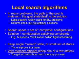
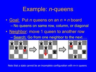
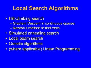
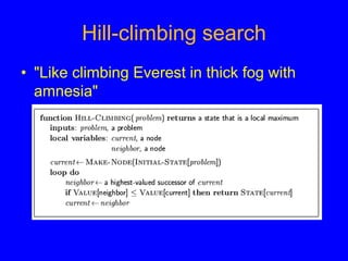
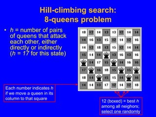
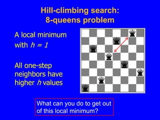
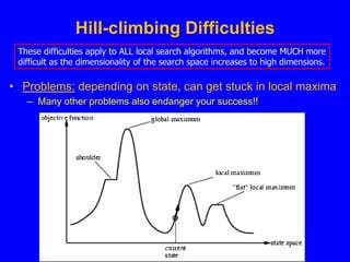
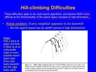
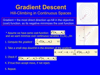
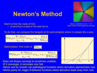
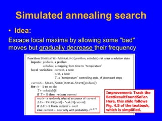
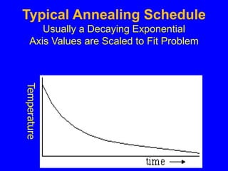
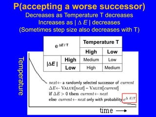
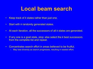
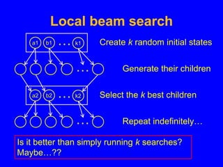
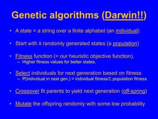
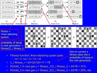
This document discusses local search algorithms. It begins by introducing the topic of local search algorithms and some examples of problems they can be applied to, such as the n-queens problem. It then describes several specific local search algorithms in more detail, including hill-climbing search, gradient descent, simulated annealing search, local beam search, and genetic algorithms. It also discusses techniques like random restart wrappers and tabu search wrappers that can help local search algorithms avoid getting stuck in local optima.

1. Local Search Algorithms
This lecture topic
Read Chapter 4.1-4.2
Next lecture topic
Read Chapter 5
(Please read lecture topic material before
and after each lecture on that topic)

2. You will be expected to know
• Local Search Algorithms
– Hill-climbing search
• Gradient Descent in continuous spaces
– Simulated annealing search
– Local beam search
– Genetic algorithms
– (where applicable) Linear Programming
• Random Restart & Tabu Wrappers for above
• Difficulties: Local optima, plateaus, ridges, etc.
• Minimize cost, maximize value
Value  Constant − Cost; Cost  Constant − Value

3. Local search algorithms
• In many problems, the path to the goal is
irrelevant; the goal state itself is the solution
– Local search: Widely used for BIG problems
– Returns good, but not optimal, solutions
• Search space = set of "complete" configurations
• Solution = configuration satisfying constraints
– E.g., N-queens, VLSI layout, Airline flight scheduling
• Keep single "current" state, or small set of states.
– Try to improve it or them.
• Very memory efficient (keep one or a few states)
– You get to control how much memory you use.

4. Example: n-queens
• Goal: Put n queens on an n × n board
– No queens on same row, column, or diagonal
• Neighbor: move 1 queen to another row
– Search: Go from one neighbor to the next….
Note that a state cannot be an incomplete configuration with m<n queens

5. Algorithm Design
Considerations
• How do you represent your problem?
• What is a “complete state”?
• What is your objective function?
– How do you measure cost or value of a state?
• What is a “neighbor” of a state?
– Or, what is a “step” from one state to another?
– How can you compute a neighbor or a step?
• Are there any constraints you can exploit?

6. Random Restart Wrapper
• These are stochastic local search methods
– Different solution for each trial and initial state
• Almost every trial hits difficulties (see below)
– Most trials will not yield a good result (sadly)
• Many random restarts improve your chances
– Many “shots at goal” may, finally, get a good one
• Restart a random initial state; many times
– Report the best result found; across many trials

7. Random Restart Wrapper
BestResultFoundSoFar <- infinitely bad;
UNTIL ( you are tired of doing it ) DO {
Result <- ( local search from random initial state );
IF ( Result is better than BestResultFoundSoFar )
THEN ( set BestResultFoundSoFar to Result );
}
RETURN BestResultFoundSoFar;
Typically, “you are tired of doing it” means that some resource limit is
exceeded, e.g., number of iterations, wall clock time, CPU time, etc.
It may also mean that Result improvements are small and infrequent,
e.g., less than 0.1% Result improvement in the last week of run time.

8. Tabu Search Wrapper
• Recently visited states added to a tabu-list
– Temporarily excluded from being visited again.
• Force solver away from explored regions
– (In principle) avoids getting stuck in local minima.
• Implemented as Hash table + FIFO queue
– Unit time cost per step; constant memory cost.
• You control how much memory is used
– Run close to the edge but don’t blow out.

9. Tabu Search Wrapper
UNTIL ( you are tired of doing it ) DO {
set Neighbor to makeNeighbor( CurrentState );
IF ( Neighbor is in HASH ) THEN ( discard Neighbor );
ELSE { push Neighbor onto FIFO, pop OldestState;
remove OldestState from HASH, insert Neighbor;
set CurrentState to Neighbor;
run yourFavoriteLocalSearch on CurrentState; } }
FIFO QUEUE
Oldest
State
New
State
HASH TABLE
State
Present?

10. Local Search Algorithms
• Hill-climbing search
– Gradient Descent in continuous spaces
– Newton’s method to find roots
• Simulated annealing search
• Local beam search
• Genetic algorithms
• (where applicable) Linear Programming

11. Hill-climbing search
• "Like climbing Everest in thick fog with
amnesia"

12. Hill-climbing search:
8-queens problem
• h = number of pairs
of queens that attack
each other, either
directly or indirectly
(h = 17 for this state)
Each number indicates h
if we move a queen in its
column to that square
12 (boxed) = best h
among all neighors;
select one randomly

13. Hill-climbing search:
8-queens problem
A local minimum
with h = 1
All one-step
neighbors have
higher h values
What can you do to get out
of this local minimum?

14. Hill-climbing Difficulties
• Problems: depending on state, can get stuck in local maxima
– Many other problems also endanger your success!!
These difficulties apply to ALL local search algorithms, and become MUCH more
difficult as the dimensionality of the search space increases to high dimensions.

15. Hill-climbing Difficulties
• Ridge problem: Every neighbor appears to be downhill
– But the search space has an uphill!! (worse in high dimensions)
These difficulties apply to ALL local search algorithms, and become MUCH more
difficult as the dimensionality of the search space increases to high dimensions.
Ridge:
Fold a piece of
paper and hold
it tilted up at an
unfavorable
angle to every
possible search
space step.
Every step
leads downhill;
but the ridge
leads uphill.

16. Gradient Descent
Hill-Climbing in Continuous Spaces
* Assume we have some cost-function:
and we want minimize over continuous variables X1,X2,..,Xn
1. Compute the gradient :
2. Take a small step downhill in the direction of the gradient:
3. Check if
4. If true then accept move, if not reject.
5. Repeat.
1
( ,..., )
n
C x x
1
( ,..., )
n
i
C x x i
x



1
' ( ,..., )
i i i n
i
x x x C x x i
x


   

1 1
( ,.., ',.., ) ( ,.., ,.., )
i n i n
C x x x C x x x

Gradient = the most direct direction up-hill in the objective
(cost) function, so its negative minimizes the cost function.

17. Gradient Descent
Hill-climbing in Continuous Spaces
• How do I determine the gradient?
– Derive formula using multivariate calculus.
– Ask a mathematician or a domain expert.
– Do a literature search.
• Variations of gradient descent can improve
performance for this or that special case.
– See Numerical Recipes in C (and in other languages)
by Press, Teukolsky, Vetterling, and Flannery.
– Simulated Annealing, Linear Programming too
• Works well in smooth spaces; poorly in rough.

18. • Want to find the roots of f(x)
– A root of f(x) is a value of x for which f(x)=0.
• To do that, we compute the tangent at Xn and compute where it crosses the x-axis.
• Optimization: find roots of
•Does not always converge & sometimes unstable.
•If it converges, it converges very fast
•Works well for smooth non-pathological functions where derivative approximates root.
•Works poorly for wiggly ill-behaved functions where derivative leads away from root.
Basins of attraction for x5 − 1 = 0;
darker means more iterations to converge.
)
(
)
(
)
(
0
)
( 1
1 n
n
n
n
n
n
n
n
x
f
x
f
x
x
x
x
x
f
x
f







 


f (xn)
 
)
(
)
(
)
(
0
)
( 1
1 n
n
n
n
n
n
n
n
x
f
x
f
x
x
x
x
x
f
x
f









 

Newton’s Method

19. Simulated annealing search
• Idea:
Escape local maxima by allowing some "bad"
moves but gradually decrease their frequency
Improvement: Track the
BestResultFoundSoFar.
Here, this slide follows
Fig. 4.5 of the textbook,
which is simplified.

20. Typical Annealing Schedule
Usually a Decaying Exponential
Axis Values are Scaled to Fit Problem
Temperature

21. P(accepting a worse successor)
Decreases as Temperature T decreases
Increases as |  E | decreases
(Sometimes step size also decreases with T)
Temperature
e E / T
Temperature T
High Low
|E |
High Medium Low
Low High Medium

22. Your “random restart
wrapper” starts here.
Goal: “Ratchet” up a jagged slope
(see HW #2, prob. #5; here T = 1; cartoon is NOT to scale)
A
Value=42
B
Value=41
C
Value=45
D
Value=44
E
Value=48
F
Value=47
G
Value=51
Value
Arbitrary (Fictitious) Search Space Coordinate
You want to get
here. HOW??
This is an
illustrative
cartoon.

23. C
Value=45
E(CB)=-4
E(CD)=-1
P(CB) .018
P(CD).37
B
Value=41
E(BA)=1
E(BC)=4
P(BA)=1
P(BC)=1
Goal: “Ratchet” up a jagged slope
(see HW #2, prob. #5; here T = 1; cartoon is NOT to scale)
A
Value=42
E(AB)=-1
P(AB) .37
D
Value=44
E(DC)=1
E(DE)=4
P(DC)=1
P(DE)=1
E
Value=48
E(ED)=-4
E(EF)=-1
P(ED) .018
P(EF).37
F
Value=47
E(FE)=1
E(FG)=4
P(FE)=1
P(FG)=1
G
Value=51
E(GF)=-4
P(GF) .018
x -1 -4
ex .37 .018
Your “random
restart wrapper”
starts here.
From A you will accept a move to B with P(AB) .37.
From B you are equally likely to go to A or to C.
From C you are 20X more likely to go to D than to B.
From D you are equally likely to go to C or to E.
From E you are 20X more likely to go to F than to D.
From F you are equally likely to go to E or to G.
Remember best point you ever found (G or neighbor?).
This is an
illustrative
cartoon.

24. Properties of simulated
annealing search
• One can prove: If T decreases slowly enough, then
simulated annealing search will find a global optimum
with probability approaching 1
– However, this may take a VERY, VERY long time.
– Note that, any finite search space, RANDOM GUESSING also will
find a global optimum with probability approaching 1.
– So, ultimately this is a very weak claim.
• Often works very well in practice
– But usually VERY, VERY slow.
• Widely used in “very big” problems:
– VLSI layout, national airline scheduling, large logistics ops, etc.

25. Local beam search
• Keep track of k states rather than just one.
• Start with k randomly generated states.
• At each iteration, all the successors of all k states are generated.
• If any one is a goal state, stop; else select the k best successors
from the complete list and repeat.
• Concentrates search effort in areas believed to be fruitful.
– May lose diversity as search progresses, resulting in wasted effort.

26. Local beam search
a1 b1 k1
… Create k random initial states
… Generate their children
a2 b2 k2
… Select the k best children
… Repeat indefinitely…
Is it better than simply running k searches?
Maybe…??

27. Genetic algorithms (Darwin!!)
• A state = a string over a finite alphabet (an individual)
• Start with k randomly generated states (a population)
• Fitness function (= our heuristic objective function).
– Higher fitness values for better states.
• Select individuals for next generation based on fitness
– P(individual in next gen.) = individual fitness/ population fitness
• Crossover fit parents to yield next generation (off-spring)
• Mutate the offspring randomly with some low probability

28. fitness =
#non-attacking
queens
• Fitness function: #non-attacking queen pairs
– min = 0, max = 8 × 7/2 = 28
• _i fitness_i = 24+23+20+11 = 78
• P(child_1 in next gen.) = fitness_1/(_i fitness_i) = 24/78 = 31%
• P(child_2 in next gen.) = fitness_2/(_i fitness_i) = 23/78 = 29%; etc
probability of being
in next generation =
fitness/(_i fitness_i)
How to convert a
fitness value into a
probability of being in
the next generation.

29. Linear Programming
Efficient Optimal Solution
For a Restricted Class of Problems
Problems of the sort:
b
=
Bx
a;
Ax
:
subject to
maximize

x
cT
•Very efficient “off-the-shelves”
solvers are available for LPs.
• They quickly solve large problems
with thousands of variables.

30. Linear Programming
Constraints
• Maximize: z = c1 x1 + c2 x2 +…+ cn xn
• Primary constraints: x10, x20, …, xn0
• Arbitrary additional linear constraints:
ai1 x1 + ai2 x2 + … + ain xn  ai, (ai  0)
aj1 x1 + aj2 x2 + … + ajn xn  aj  0
bk1 x1 + bk2 x2 + … + bkn xn = bk  0
• Restricted class of linear problems.
– Efficient for very large problems(!!) in this class.

31. Summary
• Local search maintains a complete solution
– Seeks to find a consistent solution (also complete)
• Path search maintains a consistent solution
– Seeks to find a complete solution (also consistent)
• Goal of both: complete and consistent solution
– Strategy: maintain one condition, seek other
• Local search often works well on large problems
– Abandons optimality
– Always has some answer available (best found so far)