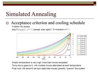
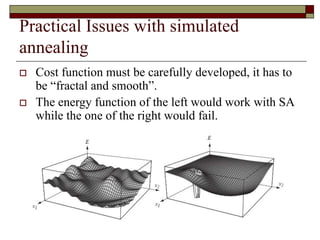
Simulated annealing is a local search algorithm that can find good approximations to global optimization problems. It is inspired by the physical process of annealing in solids. The algorithm starts with a random solution and uses the Metropolis algorithm to probabilistically accept moves to neighboring solutions based on a cooling schedule, allowing it to escape local optima. It has been applied successfully to problems like the traveling salesman problem, graph partitioning, and VLSI design placement and routing. The cost function and cooling schedule are important factors that affect its performance.

1. Simulated Annealing
10/7/2005

2. Local Search algorithms
 Search algorithms like breadth-first, depth-first or
A* explore all the search space systematically by
keeping one or more paths in memory and by
recording which alternatives have been explored.
 When a goal is found, the path to that goal
constitutes a solution.
 Local search algorithms can be very helpful if we are
interested in the solution state but not in the path to
that goal. They operate only on the current state and
move into neighboring states .

3. Local Search algorithms
 Local search algorithms have 2 key advantages:
 They use very little memory
 They can find reasonable solutions in large or infinite
(continuous) state spaces.
 Some examples of local search algorithms are:
 Hill-climbing
 Random walk
 Simulated annealing

4. Annealing
 Annealing is a thermal process for obtaining low
energy states of a solid in a heat bath.
 The process contains two steps:
 Increase the temperature of the heat bath to a maximum
value at which the solid melts.
 Decrease carefully the temperature of the heat bath until
the particles arrange themselves in the ground state of the
solid. Ground state is a minimum energy state of the solid.
 The ground state of the solid is obtained only if the
maximum temperature is high enough and the
cooling is done slowly.

5. Simulated Annealing
 The process of annealing can be simulated with the
Metropolis algorithm, which is based on Monte
Carlo techniques.
 We can apply this algorithm to generate a solution to
combinatorial optimization problems assuming an
analogy between them and physical many-particle
systems with the following equivalences:
 Solutions in the problem are equivalent to states in a
physical system.
 The cost of a solution is equivalent to the “energy” of a
state.

6. Simulated Annealing
 To apply simulated annealing with optimization purposes we
require the following:
 A successor function that returns a “close” neighboring solution given
the actual one. This will work as the “disturbance” for the particles of
the system.
 A target function to optimize that depends on the current state of the
system. This function will work as the energy of the system.
 The search is started with a randomized state. In a polling
loop we will move to neighboring states always accepting the
moves that decrease the energy while only accepting bad
moves accordingly to a probability distribution dependent on
the “temperature” of the system.

7. Simulated Annealing
 The distribution used to
decide if we accept a bad
movement is know as
Boltzman distribution.
Decrease the temperature slowly, accepting less bad moves at
each temperature level until at very low temperatures the
algorithm becomes a greedy hill-climbing algorithm.
 This distribution is very well known is in solid physics
and plays a central role in simulated annealing. Where γ
is the current configuration of the system, E γ is the
energy related with it, and Z is a normalization constant.

8. Simulated Annealing: the code
1. Create random initial solution γ
2. Eold=cost(γ);
3. for(temp=tempmax; temp>=tempmin;temp=next_temp(temp) ) {
4. for(i=0;i<imax; i++ ) {
5. succesor_func(γ); //this is a randomized function
6. Enew=cost(γ);
7. delta=Enew-Eold;
8. if(delta>0)
9. if(random() >= exp(-delta/K*temp);
10. undo_func(γ); //rejected bad move
11. else
12. Eold=Enew //accepted bad move
13. else
14. Eold=Enew; //always accept good moves
}
}

9. Simulated Annealing
 Acceptance criterion and cooling schedule

10. Practical Issues with simulated
annealing
 Cost function must be carefully developed, it has to
be “fractal and smooth”.
 The energy function of the left would work with SA
while the one of the right would fail.

11. Practical Issues with simulated
annealing
 The cost function should be fast it is going to
be called “millions” of times.
 The best is if we just have to calculate the
deltas produced by the modification instead of
traversing through all the state.
 This is dependent on the application.

12. Practical Issues with simulated
annealing
 In asymptotic convergence simulated
annealing converges to globally optimal
solutions.
 In practice, the convergence of the algorithm
depends of the cooling schedule.
 There are some suggestion about the cooling
schedule but it stills requires a lot of testing
and it usually depends on the application.

13. Practical Issues with simulated
annealing
 Start at a temperature where 50% of bad moves are
accepted.
 Each cooling step reduces the temperature by 10%
 The number of iterations at each temperature should
attempt to move between 1-10 times each “element”
of the state.
 The final temperature should not accept bad moves;
this step is known as the quenching step.

14. Applications
 Basic Problems
 Traveling salesman
 Graph partitioning
 Matching problems
 Graph coloring
 Scheduling
 Engineering
 VLSI design
 Placement
 Routing
 Array logic minimization
 Layout
 Facilities layout
 Image processing
 Code design in information theory

15. Applications: Placement
 Pick relative location for each gate.
 Seek to improve routeability, limit delay and
reduce area.
 This is achieved through the reduction of the
signals per routing channel, the balancing
row width and the reduction of wirelength.
 The placement also has to follow some
restrictions like:
 I/Os at the periphery
 Rectangular shape
 Manhattan routing
 The cost function should balance this
multiple objectives while the successor has
to comply with the restrictions.

16. Applications: Placement
 In placement there are multiple complex objective.
 The cost function is difficult to balance and requires
testing.
 An example of cost function that balances area
efficiency vs. performance.
 Cost=c1area+c2delay+c3power+c4crosstalk
 Where the ci weights heavily depend on the
application and requirements of the project

17. References
 Aarst, “Simulated annealing and Boltzman
machines”, Wiley, 1989.
 Duda Hart Stork, “Pattern Classification”, Wiley
Interscience, 2001.
 Otten, “The Annealing Algorithm”, Kluwer
Academic Publishers, 1989.
 Sherwani, “Algorithms for VLSI Physical Design
Automation”, Kluwer Academic Publishers, 1999.