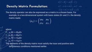
2. Ensemble
Often, if not always, our system consists of large number of
particles or our system itself can be a collection of
subsystems. This is called an Ensemble
3. Hilbert Space
In mathematics, Hilbert spaces (named after David Hilbert) allow the
methods of linear algebra and calculus to be generalized from (finite-
dimensional) Euclidean vector spaces to spaces that may be infinite-
dimensional. Hilbert spaces arise naturally and frequently in
mathematics and physics, typically as function spaces. Formally, a
Hilbert space is a vector space equipped with an inner product that
induces a distance function for which the space is a complete metric
space.
4. Density operator
A density operator, denoted by ρ, is a linear, positive semidefinite
operator on the Hilbert space of a quantum system. It encodes
the statistical ensemble of pure states that represent the
system's state of knowledge.
5. Density operator
A density operator can be expanded in terms of an orthonormal basis of
the Hilbert space:
ρ = 𝛴𝑖 𝑝𝑖| 𝜓𝑖 > < 𝜓𝑖 |
where:
• | 𝜓𝑖 > are the basis states.
• 𝑝𝑖 are the probabilities of the system being in each pure state | 𝜓𝑖 >.
• These probabilities must be non-negative and sum to 1: 𝛴𝑖 𝑝𝑖 = 1.
6. Density operator
Mathematical Properties:
• Trace: Tr(ρ) = 1 (normalized)
• Positive semidefinite: ρ ≥ 0, meaning all its eigenvalues are
non-negative.
• Hermitian: ρ = ρ† (conjugate transpose)
7. Pure vs. Mixed States:
• A pure state, represented by a ket vector |ψ>, has a density operator
given by: ρ = |ψ><ψ|
• A mixed state is a statistical mixture of pure states, often arising
from incomplete knowledge or interactions with the environment. It's
described by a density operator that is more general than a pure
state's operator.
8. Expectation Values:
The expectation value of an observable Q can be calculated using the
following formula:
<Q> = Tr(ρQ)
where Tr denotes the trace operation. This allows us to calculate average
values of observables in mixed states.
9. Density Matrix Formulation:
The density operator can also be expressed as a matrix in a chosen basis. For
example, in a two-dimensional system with basis states |0> and |1>, the density
matrix reads:
where:
• ρ_00 = <0|ρ|0>
• ρ_01 = <0|ρ|1>
• ρ_10 = <1|ρ|0>
• ρ_11 = <1|ρ|1>
The elements of the density matrix must satisfy the trace and positive semi
definiteness conditions mentioned earlier.
10. Base to Quantum computing
Qubits:
Can be in a state of 0, 1, or a superposition of both, allowing them to store multiple possibilities
simultaneously. This gives them much greater processing power compared to classical bits.
Physical realizations:
Qubits can be physically realized using various systems, including:
Electrons: Spin state (up or down) represents 0 or 1.
Photons: Polarization (horizontal or vertical) represents 0 or 1.
Atoms: Energy levels represent 0 or 1.
Superposition and its implications:
Superposition allows a qubit to represent multiple possibilities simultaneously. Imagine flipping a coin:
a classical bit would be either heads or tails, but a qubit could be "both" until measured.
This enables parallel processing of information, potentially solving problems exponentially faster than
classical computers for certain tasks.
11. Thank you
There are two kinds of statistics, the kind you look up and the
kind you make up.
~Rex Stout