In this lecture, you will learn two of the most popular methods for classifying data points into a finite set of categories. Both methods are based on representing a classifier via its decision boundary which is a hyperplane. The parameters of the hyperplane are learned from training data by minimizing a particular loss function.

1. aalto-logo-en-3
A Classification Problem
Logistic Regression
Support Vector Classification
Wrap Up
CS-E3210 Machine Learning: Basic Principles
Lecture 5: Classification I
slides by Alexander Jung, 2017
Department of Computer Science
Aalto University, School of Science
Autumn (Period I) 2017
1 / 38

2. aalto-logo-en-3
A Classification Problem
Logistic Regression
Support Vector Classification
Wrap Up
Today’s Motto
similar features give similar labels
2 / 38

3. aalto-logo-en-3
A Classification Problem
Logistic Regression
Support Vector Classification
Wrap Up
Material
this lecture is inspired by
video lectures of Andrew Ng
https://www.youtube.com/watch?v=-la3q9d7AKQ
https://www.youtube.com/watch?v=7F-CuXdTQ5k
lecture notes
http://cs229.stanford.edu/notes/cs229-notes1.pdf
Ch. 2.2 of the tutorial “Kernel Methods in Computer Vision”
by Ch. Lampert https://pub.ist.ac.at/~chl/papers/
lampert-fnt2009.pdf
lecture notes http://www.robots.ox.ac.uk/~az/
lectures/ml/lect2.pdf
3 / 38

4. aalto-logo-en-3
A Classification Problem
Logistic Regression
Support Vector Classification
Wrap Up
In A Nutshell
today we consider classification problems
consider data points z with features x and label y
want to learn classifier h(·) for predicting y based on h(x)
today we consider parametric classifiers h(w,b)
a classifier is represented by parameters w, b
we learn/find optimal parameters w, b using training data X
once we have learnt optimal parameter, we can discard data !
4 / 38

5. aalto-logo-en-3
A Classification Problem
Logistic Regression
Support Vector Classification
Wrap Up
Outline
1 A Classification Problem
2 Logistic Regression
3 Support Vector Classification
4 Wrap Up
5 / 38

6. aalto-logo-en-3
A Classification Problem
Logistic Regression
Support Vector Classification
Wrap Up
Ski Resort Marketing
you are working in the marketing agency of a ski resort
hard disk full of webcam snapshots (gigabytes of data)
want to group them into “winter” and ”summer” images
you have only a few hours for this task ...
6 / 38

7. aalto-logo-en-3
A Classification Problem
Logistic Regression
Support Vector Classification
Wrap Up
Webcam Snapshots
7 / 38

8. aalto-logo-en-3
A Classification Problem
Logistic Regression
Support Vector Classification
Wrap Up
Labeled Webcam Snapshots
create dataset X by randomly selecting N = 6 snapshots
manually categorise/label them (y(i) = 1 for summer)
8 / 38

9. aalto-logo-en-3
A Classification Problem
Logistic Regression
Support Vector Classification
Wrap Up
Towards an ML Problem
we have few labeled snapshots in X
need an algorithm/method/software-app to automatically
label all snapshots as either “winter” or “summer”
each snapshot is several MByte large
computational/time constraints force us to use more compact
representation (features)
what are good features of a snapshot for classifying summer
vs. winter?
9 / 38

10. aalto-logo-en-3
A Classification Problem
Logistic Regression
Support Vector Classification
Wrap Up
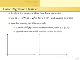
Redness, Greenness and Blueness
summer images are expected to be more colourful
winter images of Alps tend to contain much “white” (snow)
lets use redness xr , greenness xg and blueness xb
redness xr :=
j∈pixels
r[j] − (1/2)(g[j] + b[j])
greenness xg :=
j∈pixels
g[j] − (1/2)(r[j] + b[j])
blueness xb :=
j∈pixels
b[j] − (1/2)(r[j] + g[j])
r[j], g[j], b[j] denote red/green/blue intensity of pixel j
10 / 38

11. aalto-logo-en-3
A Classification Problem
Logistic Regression
Support Vector Classification
Wrap Up
A Classification Problem
labeled dataset X = {(x(i), y(i))}N
i=1
feature vector x(i) = (x
(i)
r , x
(i)
g , x
(i)
b )T ∈ R3
label y(i) = 1 for summer and y(i) = 0 for winter
find a classifier h(·) : R3 → {0, 1} with y ≈ h(x)
which hypothesis space H and loss L(z, h(·)) should we use?
11 / 38

12. aalto-logo-en-3
A Classification Problem
Logistic Regression
Support Vector Classification
Wrap Up
Linear Regression Classifier
lets first try to recycle ideas from linear regression
use H = {h(w)(x) = wT x, for w ∈ Rd } and squared error loss
two shortcomings of this approach:
classifier h(w)
(x) can be any real number, while y ∈ {0, 1}
squared error loss would penalize correct decisions
12 / 38

13. aalto-logo-en-3
A Classification Problem
Logistic Regression
Support Vector Classification
Wrap Up
Outline
1 A Classification Problem
2 Logistic Regression
3 Support Vector Classification
4 Wrap Up
13 / 38

14. aalto-logo-en-3
A Classification Problem
Logistic Regression
Support Vector Classification
Wrap Up
Taking Label Space Into Account
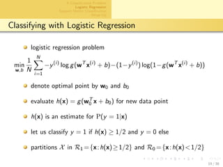
lets exploit that labels y take only values 0 or 1
use predictor h(·) with h(x) ∈ [0, 1]
one such choice is
h(w,b)
(x) = g(wT
x + b) with g(z) := 1/(1 + exp(−z))
g(z) known as logistic or sigmoid function
classifier is parametrized by weight w and offset b
14 / 38

15. aalto-logo-en-3
A Classification Problem
Logistic Regression
Support Vector Classification
Wrap Up
The Sigmoid Function
15 / 38

16. aalto-logo-en-3
A Classification Problem
Logistic Regression
Support Vector Classification
Wrap Up
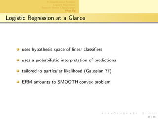
A Probabilistic Interpretation
LogReg predicts y ∈{0, 1} by h(x)=g(w ·x+b)∈[0, 1]
lets model the label y and features x as random variables
features x are given/observed/measured
conditional probabilities P{y = 1|x} and P{y = 0|x}
estimate P{y = 1|x} by h(w,b)(x)
this yields the following relation
P{y|x} = h(w,b)
(x)y
(1 − h(w,b)
(x))(1−y)
16 / 38

17. aalto-logo-en-3
A Classification Problem
Logistic Regression
Support Vector Classification
Wrap Up
Logistic Regression
max. likelihood max
w,b
P{y|x}=h(w,b)(x)y (1−h(w,b)(x))(1−y)
max. P{y|x} equivalent to min. logistic loss
L((x, y), h(w,b)
(·)) := − log P{y|x}
= −y log h(w,b)
(x)−(1−y) log(1−h(w,b)
(x))
choose w and b via empirical risk minimisation
min
w
E{h(w,b)
(·)|X} =
1
N
N
i=1
L((x(i)
, y(i)
), h(·))
=
1
N
N
i=1
−y(i)
log h(x(i)
)−(1−y(i)
) log(1−h(x(i)
))
=
1
N
N
i=1
−y(i)
log g(wT
x(i)
+ b)−(1−y(i)
) log(1−g(wT
x(i)
+ b))
17 / 38

18. aalto-logo-en-3
A Classification Problem
Logistic Regression
Support Vector Classification
Wrap Up
ID Card of Logistic Regression
input/feature space X = Rd
label space Y = [0, 1]
loss function L((x, y), h(·)) = −y log h(x)−(1−y) log(1−h(x))
hypothesis space
H = {h(w,b)(x)=g(wT x+b), with w ∈ Rd , b ∈ R}
classify y = 1 if h(w,b)(x) ≥ 0.5 and y = 0 otherwise
18 / 38

19. aalto-logo-en-3
A Classification Problem
Logistic Regression
Support Vector Classification
Wrap Up
Classifying with Logistic Regression
logistic regression problem
min
w,b
1
N
N
i=1
−y(i)
log g(wT
x(i)
+ b)−(1−y(i)
) log(1−g(wT
x(i)
+ b))
denote optimal point by w0 and b0
evaluate h(x) = g(wT
0 x + b0) for new data point
h(x) is an estimate for P(y = 1|x)
let us classify y = 1 if h(x) ≥ 1/2 and y = 0 else
partitions X in R1 ={x:h(x)≥1/2} and R0 ={x:h(x)<1/2}
19 / 38

20. aalto-logo-en-3
A Classification Problem
Logistic Regression
Support Vector Classification
Wrap Up
The Decision Boundary of Logistic Regression
20 / 38

21. aalto-logo-en-3
A Classification Problem
Logistic Regression
Support Vector Classification
Wrap Up
Learning a Logistic Regression Model
logistic regression problem
min
w,b
1
N
N
i=1
−y(i)
log g(wT
x(i)
+ b)−(1−y(i)
) log(1−g(wT
x(i)
+ b))
in contrast to LinReg, no closed-form solution here
however, we can use GD !
21 / 38

22. aalto-logo-en-3
A Classification Problem
Logistic Regression
Support Vector Classification
Wrap Up
A Learning Algorithm for Classification
input: labeled data set X, step-size or learning rate α
output: classifier h(w,b)(x) = g(wT x + b)
initalize: k := 0 and w0 := 0 and b0 := 0
until stopping criterion satisfied do
(w(k+1)
, b(k+1)
):=(w(k)
, b(k)
)−α w,bE{h(w(k)
,b(k)
)
|X}
k := k + 1
set w := w(k), b := b(k)
22 / 38

23. aalto-logo-en-3
A Classification Problem
Logistic Regression
Support Vector Classification
Wrap Up
Outline
1 A Classification Problem
2 Logistic Regression
3 Support Vector Classification
4 Wrap Up
23 / 38

24. aalto-logo-en-3
A Classification Problem
Logistic Regression
Support Vector Classification
Wrap Up
Binary Linear Classifiers
logistic regression delivers a linear classifier
linear classifier specified by normal vector w and offset b
let us from now on code the binary labels as +1 and −1
output of linear classifier ˆy = I(h(w,b)(x) > 0) with linear
predictor h(w,b)(x) = wT x + b
we can use different loss functions for learning w and b!
seemingly, squared error loss is not good for binary labels
24 / 38

25. aalto-logo-en-3
A Classification Problem
Logistic Regression
Support Vector Classification
Wrap Up
Minimizing Error Probability
eventually, we aim at low error probability P{ˆy = y}
using 0/1-loss L((x, y), h(·)) = I(ˆy = y) we can approximate
P{ˆy = y} ≈ (1/N)
N
i=1
L((x(i)
, y(i)
), h(·))
the optimal classifier is then obtained by
min
h(·)∈H
N
i=1
L((x(i)
, y(i)
), h(·))
non-convex non-smooth optimization problem ! (there is a
work-around as we see in next lecture :-)
25 / 38

26. aalto-logo-en-3
A Classification Problem
Logistic Regression
Support Vector Classification
Wrap Up
The 0/1 Loss
26 / 38

27. aalto-logo-en-3
A Classification Problem
Logistic Regression
Support Vector Classification
Wrap Up
The Hinge Loss
27 / 38

28. aalto-logo-en-3
A Classification Problem
Logistic Regression
Support Vector Classification
Wrap Up
The Hinge Loss (y = 1)
28 / 38

29. aalto-logo-en-3
A Classification Problem
Logistic Regression
Support Vector Classification
Wrap Up
The Hinge Loss (y = −1)
29 / 38

30. aalto-logo-en-3
A Classification Problem
Logistic Regression
Support Vector Classification
Wrap Up
Learning Linear Classifier via Hinge Loss
linear classifier h(w,b)(x) = wT x + b
choose w and b by minimizing hinge loss
L((x, y), h(w,b)
) = max{0, 1−y · h(w,b)
(x)}
= max{0, 1 − y · (wT
x + b)}
learn optimal classifier via empirical risk minimization
min
w,b
E(h(w,b)
|X) :=
1
N
N
i=1
L((x(i)
, y(i)
), h(w,b)
(·))
=
1
N
N
i=1
max{0, 1 − y(i)
(wT
x(i)
+ b)}
30 / 38

31. aalto-logo-en-3
A Classification Problem
Logistic Regression
Support Vector Classification
Wrap Up
SVC Maximizes Margin
we can rewrite hinge loss as
L((x, y), h(w,b)
) = max{0, 1 − y · (wT
x + b)}
= min
ξ≥0
ξ s.t. ξ ≥ 1 − y · (wT
x + b)
“margin
minimizing hing loss means maximizing margin
min
w,b
E(h(w,b)
|X) =
1
N
N
i=1
max{0, 1 − y(i)
(wT
x(i)
+ b)}
=
1
N
min
ξ(i)≥0
N
i=1
ξ(i)
s.t. ξ(i)
≥ 1 − y(i)
· (wT
x(i)
+ b)
31 / 38

32. aalto-logo-en-3
A Classification Problem
Logistic Regression
Support Vector Classification
Wrap Up
SVC Maximizes Margin
32 / 38

33. aalto-logo-en-3
A Classification Problem
Logistic Regression
Support Vector Classification
Wrap Up
ID Card of Support Vector Classifier
input/feature space X = Rd
label space Y = {−1, 1}
loss function L((x, y), h(·)) = max{0, 1 − y · h(w,b)(x)}
hypothesis space
H = {h(w,b)(x)=wT x+b, with w ∈ Rd , b ∈ R}
classify y = 1 if h(w,b)(x) ≥ 0 and y = −1 else
33 / 38

34. aalto-logo-en-3
A Classification Problem
Logistic Regression
Support Vector Classification
Wrap Up
Outline
1 A Classification Problem
2 Logistic Regression
3 Support Vector Classification
4 Wrap Up
34 / 38

35. aalto-logo-en-3
A Classification Problem
Logistic Regression
Support Vector Classification
Wrap Up
What We Learned Today
how to formulize a classification problem
different loss functions yield different classification methods
LogReg with logistic loss; amounts to maximum likelihood
SVC with hinge-loss and amounts to max. margin
LogReg and SVC are both parametric and linear classifiers
35 / 38

36. aalto-logo-en-3
A Classification Problem
Logistic Regression
Support Vector Classification
Wrap Up
Logistic Regression at a Glance
uses hypothesis space of linear classifiers
uses a probabilistic interpretation of predictions
tailored to particular likelihood (Gaussian ??)
ERM amounts to SMOOTH convex problem
36 / 38

37. aalto-logo-en-3
A Classification Problem
Logistic Regression
Support Vector Classification
Wrap Up
Support Vector Classifier (Machine) at a Glance
uses hypothesis space of linear classifiers
based on geometry (maximum margin between classes)
can be extended by using feature methods (kernel methods)
ERM amounts to NON-SMOOTH cvx opt problem
37 / 38

38. aalto-logo-en-3
A Classification Problem
Logistic Regression
Support Vector Classification
Wrap Up
What Happens Next?
next lecture on two further classification methods (decision
trees and naive Bayes)
read Sec. 9.2 - 9.2.3 of
https://web.stanford.edu/~hastie/Papers/ESLII.pdf
fill out post-lecture questionnaire in MyCourses (contributes
to grade!)
38 / 38