Download as PDF, PPTX
![THE IDEA OF GRAPH CONVOLUTIONAL NETWORKS (GCN)THE IDEA OF GRAPH CONVOLUTIONAL NETWORKS (GCN)
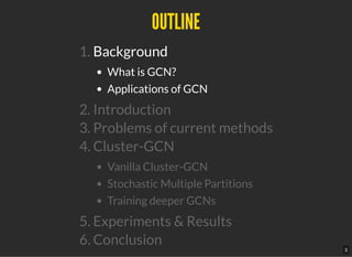
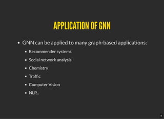
First, change the feature vector into a list of N feature vectors (a feature matrix)
So, at each layer , we N nodes, each node is represented by a feature vector [i]
One more idea: Take the relationship of nodes into account
In graph, one way to represent the relationship of nodes is to use adjacency matrix
The transformation at layer become
One way to de ne :
So, we have:
Intuition: accumulate features from the neighbors before applying the transformation
In fact, A can be normalized in some way before using, e.g., augment self feature, divided by degree matrix...
∈X
(l)
ℝ
1×Fl
∈X
(l)
ℝ
N×Fl
l
th
i
th
X
(l)
A ∈ ℝ
N×N
l
th
= f (A, , )Z
(l+1)
X
(l)
W
(l)
f
f (A, , ) = AX
(l)
W
(l)
X
(l)
W
(l)
= A , = σ( )Z
(l+1)
X
(l)
W
(l)
X
(l+1)
Z
(l+1)
W
(l)
5](https://image.slidesharecdn.com/vjai-paperreading3-kdd2019-clustergcn-190818140655/85/VJAI-Paper-Reading-3-KDD2019-ClusterGCN-5-320.jpg)
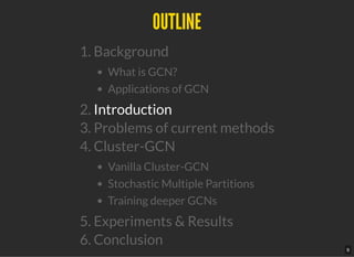
![INTRODUCTIONINTRODUCTION
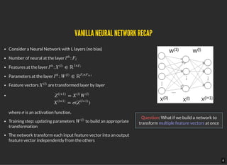
Computational cost of current SGD-based algorithms exponentially grows with
number of layers.
Large space requirement for keeping the entire graph and the embedding of each
node in memory.
Propose Cluster-GCN [1] that exploits the graph clustering structure:
Samples a block of nodes that associate with a dense subgraph identi edby a graph clustering
algorithm
Restricts the neighborhood search within this subgraph
Cluster-GCN signi cantly improved memory and computational ef ciency, which
allows us to train much deeper GCN without much time and memory overhead.
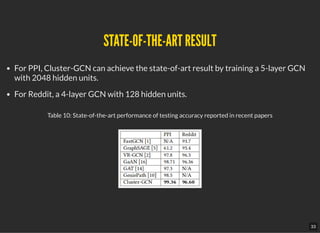
5-layer Cluster-GCN achieves state-of-the-art test F1 score 99.36 on the PPI
dataset (the previous best result was 98.71)
[ ], [ ]Paper Code
10](https://image.slidesharecdn.com/vjai-paperreading3-kdd2019-clustergcn-190818140655/85/VJAI-Paper-Reading-3-KDD2019-ClusterGCN-10-320.jpg)
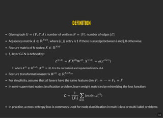
![FULL-BATCH GRADIENT DESCENT (FROM [2])FULL-BATCH GRADIENT DESCENT (FROM [2])
Store all the embedding matrices
→ Memory problem
Update the model once per epoch
→ require more epochs to converge
{Z
(l)
}
L
l=1
13](https://image.slidesharecdn.com/vjai-paperreading3-kdd2019-clustergcn-190818140655/85/VJAI-Paper-Reading-3-KDD2019-ClusterGCN-13-320.jpg)
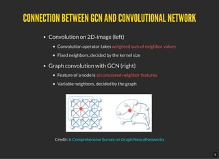
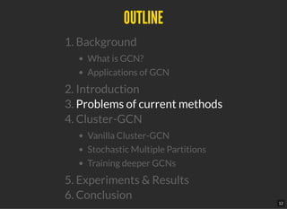
![MINI-BATCH SGD (FROM [3])MINI-BATCH SGD (FROM [3])
Update model for each batch of nodes
Signi cant computational overhead due to neighborhood
expansion problem
Converge faster in terms of epochs but much slower per-epoch
training time
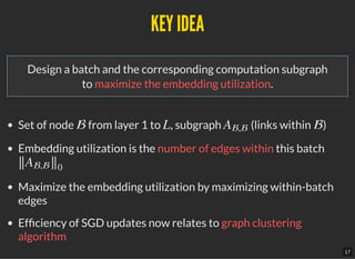
Embedding utilization:
If the node ’s embedding at -th layer is computed and is reused times
for the embedding computations at layer ,
then we say the embedding utilization of is .
Embedding utilization u is small because graph is usually large and
sparse
i l z
(l)
i
u
l + 1
z
(l)
i
u
14](https://image.slidesharecdn.com/vjai-paperreading3-kdd2019-clustergcn-190818140655/85/VJAI-Paper-Reading-3-KDD2019-ClusterGCN-14-320.jpg)
![VR-GCN (FROM [4]) (SOTA)VR-GCN (FROM [4]) (SOTA)
Reduce the size of neighborhood sampling nodes
Requires storing all the intermediate embeddings
15](https://image.slidesharecdn.com/vjai-paperreading3-kdd2019-clustergcn-190818140655/85/VJAI-Paper-Reading-3-KDD2019-ClusterGCN-15-320.jpg)
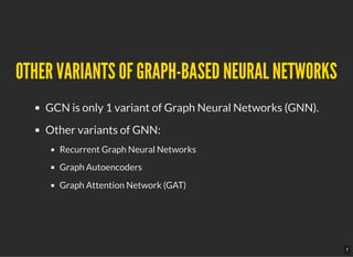
![GRAPH PARTITIONINGGRAPH PARTITIONING
Partition the graph into c groups: , where consists of the nodes in the -th partition.
only consists of the links between nodes in .
Adjacencty matrix A is partitioned into submatrices as:
Also partition feature X and training labels Y according to as and
G = [ , · · · ]1 c t t
= [ , · · ·, ] = [{ , }, · · ·, {V c, }]G¯ G1 Gc 1 1 c
t t
c
2
A = + Δ =A¯
⎡
⎣
⎢
⎢
⎢
A11
⋮
Ac1
⋯
⋱
⋯
A1c
⋮
Acc
⎤
⎦
⎥
⎥
⎥
where = , Δ =A¯
⎡
⎣
⎢
⎢
⎢
A11
⋮
0
⋯
⋱
⋯
0
⋮
Acc
⎤
⎦
⎥
⎥
⎥
⎡
⎣
⎢
⎢
⎢
0
⋮
Ac1
⋯
⋱
⋯
A1c
⋮
0
⎤
⎦
⎥
⎥
⎥
[ , · · · ]1 c [ , · · ·, ]X1 Xc [ , · · ·, ]Y1 Yc
18](https://image.slidesharecdn.com/vjai-paperreading3-kdd2019-clustergcn-190818140655/85/VJAI-Paper-Reading-3-KDD2019-ClusterGCN-18-320.jpg)
![Table 3: Data statistics Table 4: The parameters used in the experiments
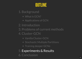
EXPERIMENTSEXPERIMENTS
Evaluate on multi-label and multi-class class ciation on 4 public datasets
Compare with 2 SoTA methods
VR-GCN (from [4]): maintains historical embedding & expands to only a few neighbors
GraphSAGE (from [5]): samples a xed number of neighbors per node.
Cluster-GCN:
Implemented with PyTorch (Google Research, why PyTorch?)
Adam optimizer, learning rate = 0.1, dropout rate=20%, zero weight decay
Number of partitions and clusters per batch are stated in Table 4.
All the experiments are run on 1 machine with NVIDIA Tesla V100 GPU (16GB
mem), 20-core Intel Xeon CPU (2.20 GHz), and 192 GB of RAM.
26](https://image.slidesharecdn.com/vjai-paperreading3-kdd2019-clustergcn-190818140655/85/VJAI-Paper-Reading-3-KDD2019-ClusterGCN-26-320.jpg)
![REFERENCESREFERENCES
[1] Wei-Lin Chiang et. al., KDD 2019. Cluster-GCN: An Ef cient Algorithm for Training Deep and Large
Graph Convolutional Networks
[2] Thomas N. Kipf and Max Welling. ICLR 2017. Semi-Supervised Classi cation with Graph Convolutional
Networks.
[3] William L. Hamilton, Rex Ying, and Jure Leskovec. NIPS 2017. Inductive Representation Learning on
Large Graphs.
[4] Jianfei Chen, Jun Zhu, and Song Le. ICML 2018. Stochastic Training of Graph Convolutional Networks
with Variance Reduction.
36](https://image.slidesharecdn.com/vjai-paperreading3-kdd2019-clustergcn-190818140655/85/VJAI-Paper-Reading-3-KDD2019-ClusterGCN-36-320.jpg)


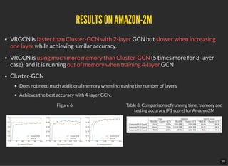
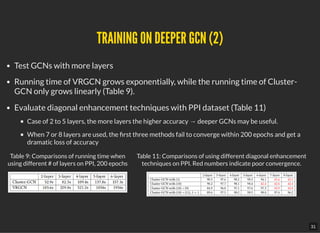
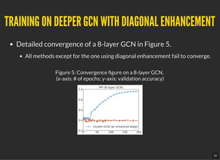
The document discusses Cluster-GCN, an efficient algorithm designed to train deep and large graph convolutional networks (GCNs) by exploiting graph clustering structures to enhance memory and computational efficiency. It addresses the limitations of current methods, presents experimental results indicating improved performance on benchmark datasets, and highlights its advantages over existing algorithms in terms of speed and memory usage. Additionally, it introduces techniques like stochastic multiple partitions and diagonal enhancement to further optimize training deeper GCNs.


![[DL輪読会]The Neural Process Family−Neural Processes関連の実装を読んで動かしてみる−](https://cdn.slidesharecdn.com/ss_thumbnails/20190415dlhacks-190422075753-thumbnail.jpg?width=640&height=640&fit=bounds)


![[DL輪読会]Encoder-Decoder with Atrous Separable Convolution for Semantic Image S...](https://cdn.slidesharecdn.com/ss_thumbnails/deeplabv3-180309001425-thumbnail.jpg?width=640&height=640&fit=bounds)


![250811_Thien_Labseminar[Cluster-GCN].pptx](https://cdn.slidesharecdn.com/ss_thumbnails/250811thienlabseminarcluster-gcn-250811132418-bc93d047-thumbnail.jpg?width=640&height=640&fit=bounds)


![[NS][Lab_Seminar_240710]Improving Graph Networks through Selection-based Conv...](https://cdn.slidesharecdn.com/ss_thumbnails/nslabseminar240710selgcn-240723105252-3f46ad9d-thumbnail.jpg?width=640&height=640&fit=bounds)