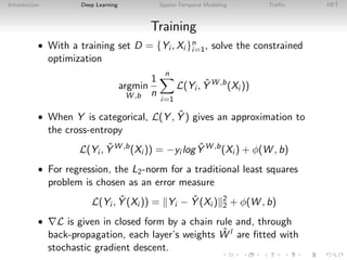
This document introduces deep learning approaches for predicting spatio-temporal flows. It discusses how deep learning uses hierarchical layers to model complex nonlinear relationships in spatial and temporal data without assuming a data generation process. Examples are given of applying deep learning to predict traffic flows using loop detector data and to forecast stock price movements using limit order book imbalances. The document outlines the configuration of deep learning models for these tasks and evaluates their performance versus traditional statistical approaches.

1. Introduction Deep Learning Spatio-Temporal Modeling Traffic HFT
Prediction of Spatio-Temporal Flows with Deep
Learning
Matthew Dixon1 2
Illinois Institute of Technology
October 11th, 2017
CISC Lunchtime Matchmaking Seminars
1
M.F. Dixon, N. Polson and V. Sokolov, Deep Learning for Spatio-Temporal
Modeling: Dynamic Traffic Flows and High Frequency Trading, arXiv:1705.09851
2
M.F. Dixon, Sequence Classification of the Limit Order Book using Recurrent
Neural Networks, to appear in J. Computational Science, Special Issue on Topics in
Computational and Algorithmic Finance, arXiv:1707.05642

2. Introduction Deep Learning Spatio-Temporal Modeling Traffic HFT
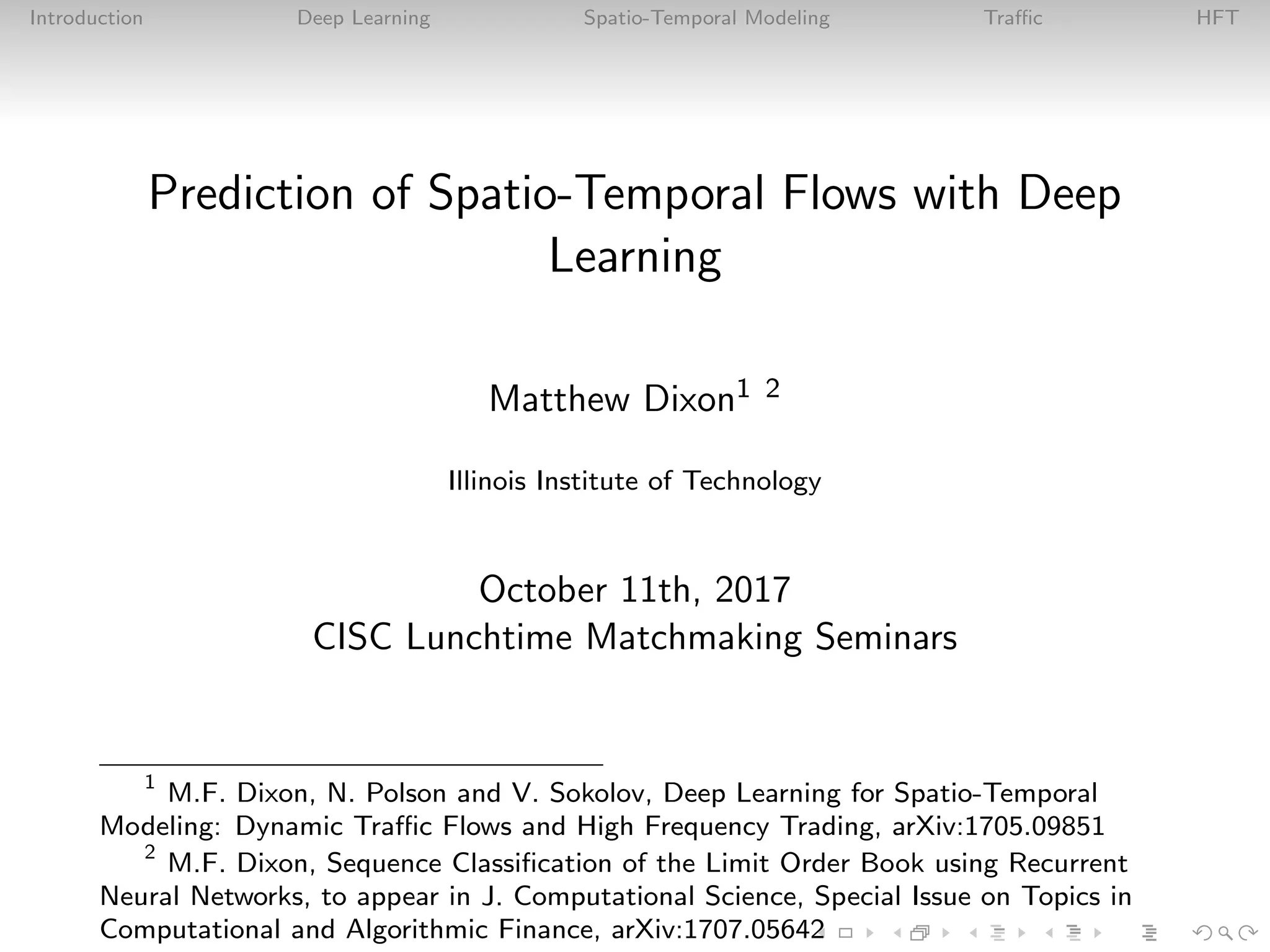
Introduction to Deep Learning
• Machine learning falls into the algorithmic class [Breiman,
2001] of reduced model estimation procedures which treats
the data generation process as an unknown.
• Deep learning is a form of machine learning that uses
hierarchical layers of abstraction to represent high-dimensional
nonlinear predictors.
• Traditional fit metrics, such as R2, t−values, p-values, and
the notion of statistical significance has been replaced in the
machine learning literature by out-of-sample forecasting and
understanding the bias-variance trade-off.
• Deep learning is data-driven and focuses on finding structure
in large data sets. The main tools for variable or predictor
selection are regularization and dropout.

3. Introduction Deep Learning Spatio-Temporal Modeling Traffic HFT
Deep Architectures in TensorFlow
feed forward auto-encoder convolution
recurrent Long / short term memory neural Turing machines
Figure: Most commonly used deep learning architectures for modeling. Source:
http://www.asimovinstitute.org/neural-network-zoo

4. Introduction Deep Learning Spatio-Temporal Modeling Traffic HFT
Growth of TensorFlow
Tensorflow
build
for
Intel
Xeon
Phi:
h6ps://github.com/tensorflow/
tensorflow.git
Source
:
Andrej
Karpathy‘s
arXiv-­‐sanity
database
• Python examples: https://github.com/Quiota/tensorflow
• R examples: 2017 Google Summer of Code Statistical Computing
Project in R (with Lan Wei), https://github.com/lweicdsor/OSTSC

5. Introduction Deep Learning Spatio-Temporal Modeling Traffic HFT
Machine Learning
• Machine learning addresses a fundamental prediction problem:
Construct a nonlinear predictor, ˆY (X), of an output, Y , given
a high dimensional input matrix3 X = (X1, . . . , XP) of P
variables.
• Machine learning can be simply viewed as the study and
construction of an input-output map of the form
Y = F(X) where X = (X1, . . . , XP).
• The output variable, Y , can be continuous, discrete or mixed.
• For example, in a classification problem, F : X → Y where
Y ∈ {1, . . . , K} and K is the number of categories. When Y
is a continuous vector and f is a semi-affine function, then we
recover the linear model
Y = AX + b.
3
With abuse of notation, X is hereon used to denote an observation matrix
of a random vector.

6. Introduction Deep Learning Spatio-Temporal Modeling Traffic HFT
Deep Predictors
Definition (Deep Predictor)
A deep predictor is a particular class of multivariate function F(X)
constructed using a sequence of L layers via a composite map
ˆY (X) := FW ,b(X) = f L
W L,bL . . . ◦ f 1
W 1,b1 (X).
• f l
W l ,bl (X) := f l (W l X + bl ) is a semi-affine function, where f l
is univariate and continuous.
• W = (W 1, . . . , W L) and b = (b1, . . . , bL) are weight matrices
and offsets respectively.
• Many statistical techniques are ’shallow learners’, e.g. PCA
Y = f (X) = WX + b, columns of W form an orthogonal
basis.

7. Introduction Deep Learning Spatio-Temporal Modeling Traffic HFT
Deep Predictors
• The structure of a deep prediction rule can be written as a
hierarchy of L − 1 unobserved layers, Zl , given by
ˆY (X) = f L
(ZL−1
),
Z0
= X,
Z1
= f 1
W 1
Z0
+ b1
,
Z2
= f 2
W 2
Z1
+ b2
,
. . .
ZL−1
= f L−1
W L−1
ZL−2
+ bL−1
.
• When Y is numeric, the output function f L(X) is given by the
semi-affine function f L(X) := f L
W L,bL (X).
• When Y is categorical, f L(X) is a softmax function.
• f (x) are ’activation’ functions, e.g. tanh(x), rectified linear
unit max(x, 0).

8. Introduction Deep Learning Spatio-Temporal Modeling Traffic HFT
Why use hidden layers?
Problem: classify whether the curve is red or blue Solution using a linear method
Figure: Image source: Chris Olah, Google Brain.

9. Introduction Deep Learning Spatio-Temporal Modeling Traffic HFT
Why use hidden layers?
Answer: To perform translations of the input space that enable
linear separability.
Transformation of the input space Result of classification using a hidden layer
using a hidden layer
Figure: Image source: Chris Olah, Google Brain.

10. Introduction Deep Learning Spatio-Temporal Modeling Traffic HFT
Training
• With a training set D = {Yi , Xi }n
i=1, solve the constrained
optimization
argmin
W ,b
1
n
n
i=1
L(Yi , ˆY W ,b
(Xi ))
• When Y is categorical, L(Y , ˆY ) gives an approximation to
the cross-entropy
L(Yi , ˆY W ,b
(Xi )) = −yi log ˆY W ,b
(Xi ) + φ(W , b)
• For regression, the L2-norm for a traditional least squares
problem is chosen as an error measure
L(Yi , ˆY (Xi )) = Yi − ˆY (Xi ) 2
2 + φ(W , b)
• L is given in closed form by a chain rule and, through
back-propagation, each layer’s weights ˆW l are fitted with
stochastic gradient descent.

11. Introduction Deep Learning Spatio-Temporal Modeling Traffic HFT
Spatial-Temporal Representation
• Cressie and Wikle (2015) provide a good overview of the
spatio-temporal modeling
• In a statistical framework, the non-parametric approach seeks
to approximate the unknown map F using a family of spatial
basic functions Φ(x) and random temporal effects w(t)
Ft(x) =
N
k=1
wk(t)φk(x)
• Gaussian processes, for spatio-temporal analysis, are
computationally intractable and assumes prior knowledge of
the covariance function.
• Convolution methods address these issues and are, in fact, a
single layer convolution network.

12. Introduction Deep Learning Spatio-Temporal Modeling Traffic HFT
Space-Temporal Representation
Figure: (left) Spatial basis functions on R2
. (right) Y = Ft(x) at time t0.

13. Introduction Deep Learning Spatio-Temporal Modeling Traffic HFT
Spatial-Temporal Neural Networks
• Construct layers as a time ”filter” given by
zl+1
i = f
Nl
i=1
(wl+1
i zl
i + bl+1
i )
• f is the activation function and Nl is the number of neurons
in layer l.

14. Introduction Deep Learning Spatio-Temporal Modeling Traffic HFT
Space-Time Diagram of Traffic

15. Introduction Deep Learning Spatio-Temporal Modeling Traffic HFT
Traffic Prediction
• Predict the traffic flow speeds at loop detector locations:
Y = xt
t+h =



x1,t+h
...
xn,t+h


 ,
• xt
t+h is the forecast of traffic flow speeds at time t + h, given
measurements up to time t.
• n is the number of locations on the network (loop detectors)
and
• xi,t is the cross-section traffic flow speed at location i at time
t

16. Introduction Deep Learning Spatio-Temporal Modeling Traffic HFT
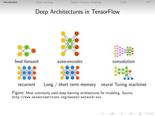
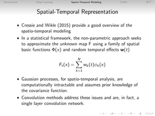
Traffic on I-55 near Chicago
0
20
40
60
0 5 10 15 20
Time [hour]
Speed[mph]
0
20
40
60
0 5 10 15 20
Time [hours]
Speed[mph]
(a) Chicago Bears football game (b) Snow weather
Figure: Impact of non-recurrent events on traffic flows. Left panel (a) shows traffic flow on a day when New
York Giants played at Chicago Bears on Thursday October 10, 2013. Right panel (b) shoes impact of light snow on
traffic flow on I-55 near Chicago on December 11, 2013. On both panels average traffic speed is red line and speed
on event day is blue line.

17. Introduction Deep Learning Spatio-Temporal Modeling Traffic HFT
Spatial-Temporal Representation in HFT
Figure: A space-time diagram showing the limit order book. The contemporaneous depths imbalances at each
price level, xi,t , are represented by the color scale: red denotes a high value of the depth imbalance and yellow the
converse. The limit order book are observed to polarize prior to a price movement.

18. Introduction Deep Learning Spatio-Temporal Modeling Traffic HFT
Limit Order Book Update Intensity
0e+00
1e+05
2e+05
3e+05
4e+05
6−7am
7−8am
8−9am
9−10am
10−11am
11−12pm
12−1pm
1−2pm
2−3pm
3−4pm
hour
Bookupdates/hour
uncertainty
Median
Figure: The hourly limit order book rates of ESU6 are shown by time of day. A surge
of quote adjustment and trading activity is consistently observed between the hours of
7-8am CST and 3-4pm CST.

19. Introduction Deep Learning Spatio-Temporal Modeling Traffic HFT
Historical data
• At any point in time, the amount of liquidity in the market
can be characterized by the cross-section of book depths.
• We build a mid-price forecasting model based on the
cross-section of book depths.
Timestamp pb
1,t pb
2,t . . . db
1,t db
2,t . . . pa
1,t pa
2,t . . . da
1,t da
2,t . . . Response
06:00:00.015 2175.75 2175.5 . . . 103 177 . . . 2176 2176.25 . . . 82 162 . . . -1
06:00:00.036 2175.5 2175.25 . . . 177 132 . . . 2175.75 2176 . . . 23 82 . . . 0
Table: The spatio-temporal representation of the limit order book before and after the arrival of the sell market
order. The response represents the direction of the mid-price movement over the subsequent interval. pb
i,t and db
i,t
denote the level i quoted bid price and depth of the limit order book at time t. pa
i,t and da
i,t denote the
corresponding level i quoted ask price and depth.

20. Introduction Deep Learning Spatio-Temporal Modeling Traffic HFT
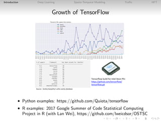
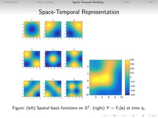
Price prediction
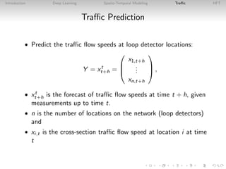
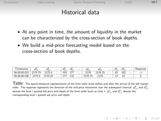
• The response is
Y = ∆pt
t+h (1)
• ∆pt
t+h is the forecast of discrete mid-price changes from time
t to t + h, given measurement of the predictors up to time t.
• The predictors are embedded
x = xt
= vec



x1,t−k . . . x1,t
...
...
xn,t−k . . . xn,t


 (2)
• n is the number of quoted price levels, k is the number of
lagged observations, and xi,t ∈ [0, 1] is the relative depth,
representing liquidity imbalance, at quote level i:
xi,t =
da
i,t
da
i,t + db
i,t
. (3)

21. Introduction Deep Learning Spatio-Temporal Modeling Traffic HFT
Model Configuration4
Activation function: f ∈ {ReLU(x), softmax(x)}
Number of hidden layers: L ∈ {3, . . . , 7}
Number of nodes in each layer: Nl ∈ {50, . . . , 200}
L1 regularization: λ1 ∈ {10−3
, 10−2
, 10−1
}
L2 regularization: λ2 ∈ {10−3
, 10−2
, 10−1
}
Learning rate: γ ∈ {10−4
, 10−3
, 10−2
}
4
Times series cross-validation is performed using an unbalanced validation and test set, each of size 2 × 105
observations. Each experiment is run for 2500 epochs with a mini-batch size of 32 drawn from the training set of
298,062 observations, containing 411 variables chosen from the elastic-net method.

22. Introduction Deep Learning Spatio-Temporal Modeling Traffic HFT
The Bias-Variance Tradeoff
(a) DNN F1-score of ˆY = 1 (b) DNN F1-score of ˆY = 0 (b) DNN F1-score of ˆY = −1.
Table: The learning curves of the deep learner are used to assess the bias-variance tradeoff and are shown for
(left) downward, (middle) neutral, or (right) upward price prediction. The variance is observed to reduce with an
increased training set size and shows that the deep learning is not-overfitting. The bias on the test set is also
observed to reduce with increased training set size.

23. Introduction Deep Learning Spatio-Temporal Modeling Traffic HFT
Receiver Operator Characteristics
(a) ROC curves of ˆY = 1 (b) ROC curves of ˆY = 0 (b) ROC curves of ˆY = −1.
Table: The Receiver Operator Characteristic (ROC) curves of the deep learner and the elastic net method are
shown for (left) downward, (middle) neutral, or (right) upward next price movement prediction.

24. Introduction Deep Learning Spatio-Temporal Modeling Traffic HFT
Prediction Example

25. Introduction Deep Learning Spatio-Temporal Modeling Traffic HFT
Summary
• Predicting spatio-temporal flows is a challenging problem as
dynamic spatio-temporal data possess underlying complex
interactions and nonlinearities
• Traditional statistical modeling approaches to spatio-temporal
modeling use a data generating process, generally motivated
by physical laws or constraints.
• Deep learning applies layers of hierarchical hidden variables to
capture these interactions and nonlinearities without using a
data generating process.
• Deep learning is able to capture sharp movements in
spatio-temporal flows without the need for smoothing.

26. Introduction Deep Learning Spatio-Temporal Modeling Traffic HFT
Remote sensing

27. Introduction Deep Learning Spatio-Temporal Modeling Traffic HFT
Next steps
• How can deep learning be used for uncertainty quantification
in spatio-temporal flows? (With Yulia Gel (University of
Texas), Vadim Sokolov (GMU) )
• New modeling approaches for insurance programs and
products linked to spatio-temporal effects such as
precipitation, drought, climate change, disease, house prices,
unemployment rates? Federal agencies (Freddie Mac, Fannie
Mae, FEMA, USDA) in addition to OFR
• NSF programs in big data, climate modeling (deadlines in
early 2018)
• NIH programs in big data and epidemiology?
• Other sponsored research programs that are related to
your area of interest?