Downloaded 352 times
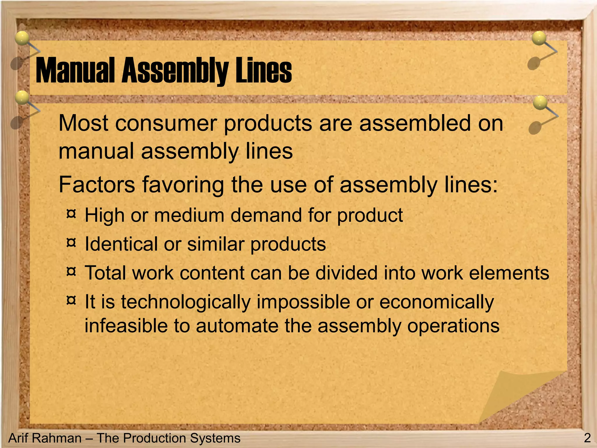
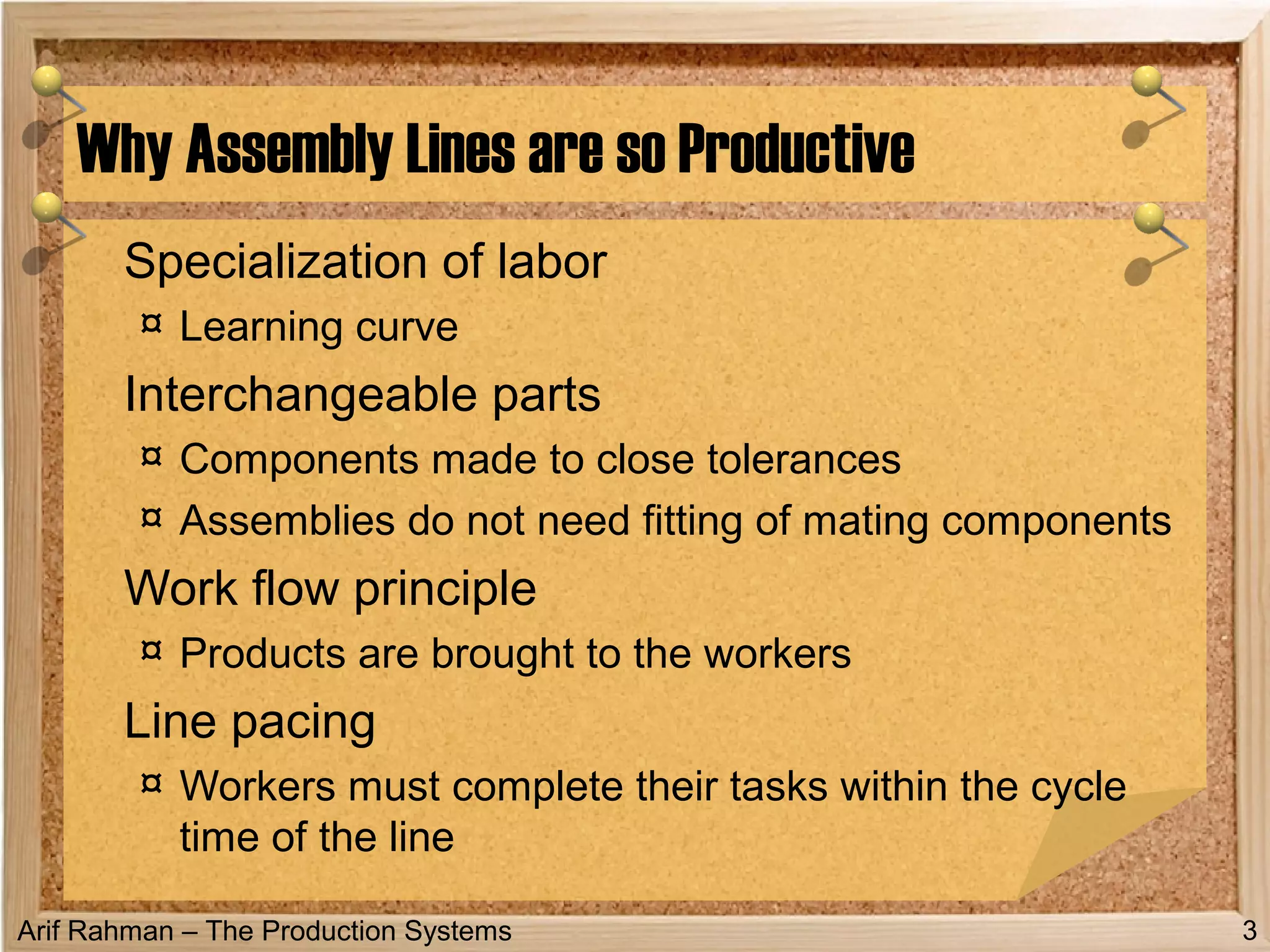
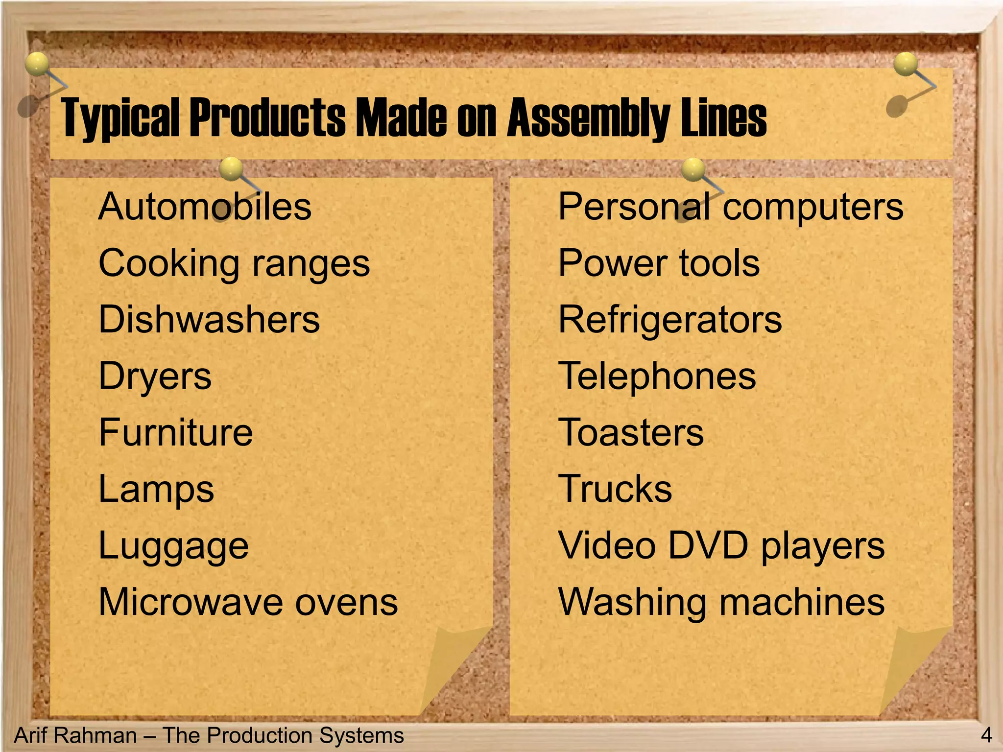
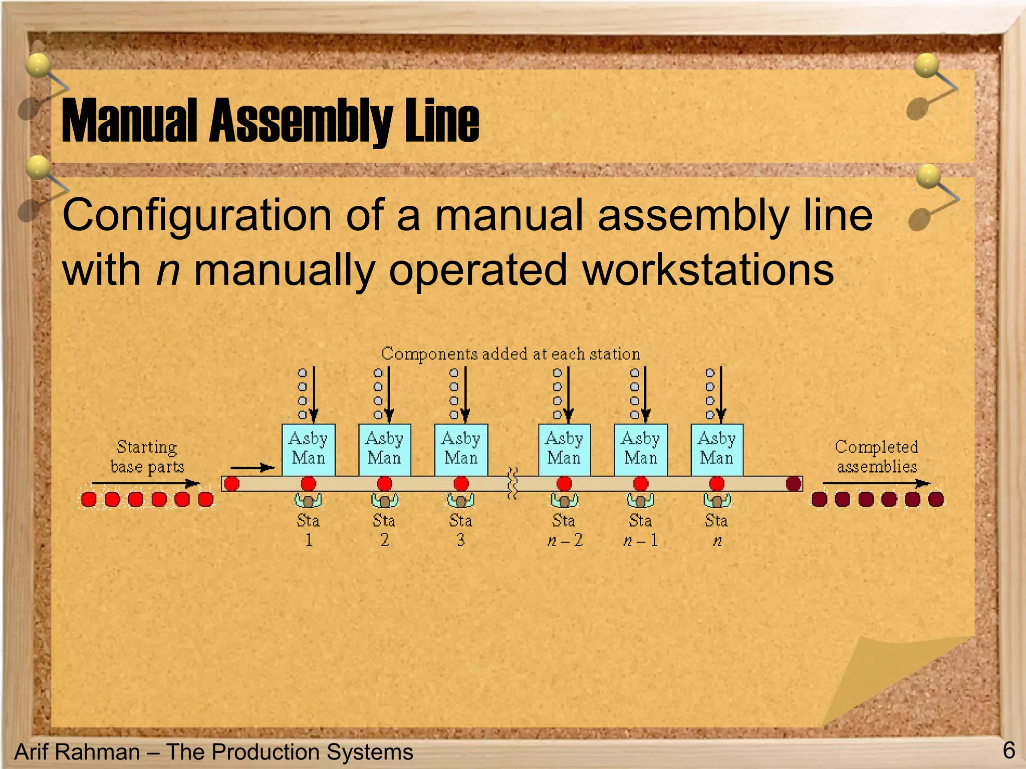


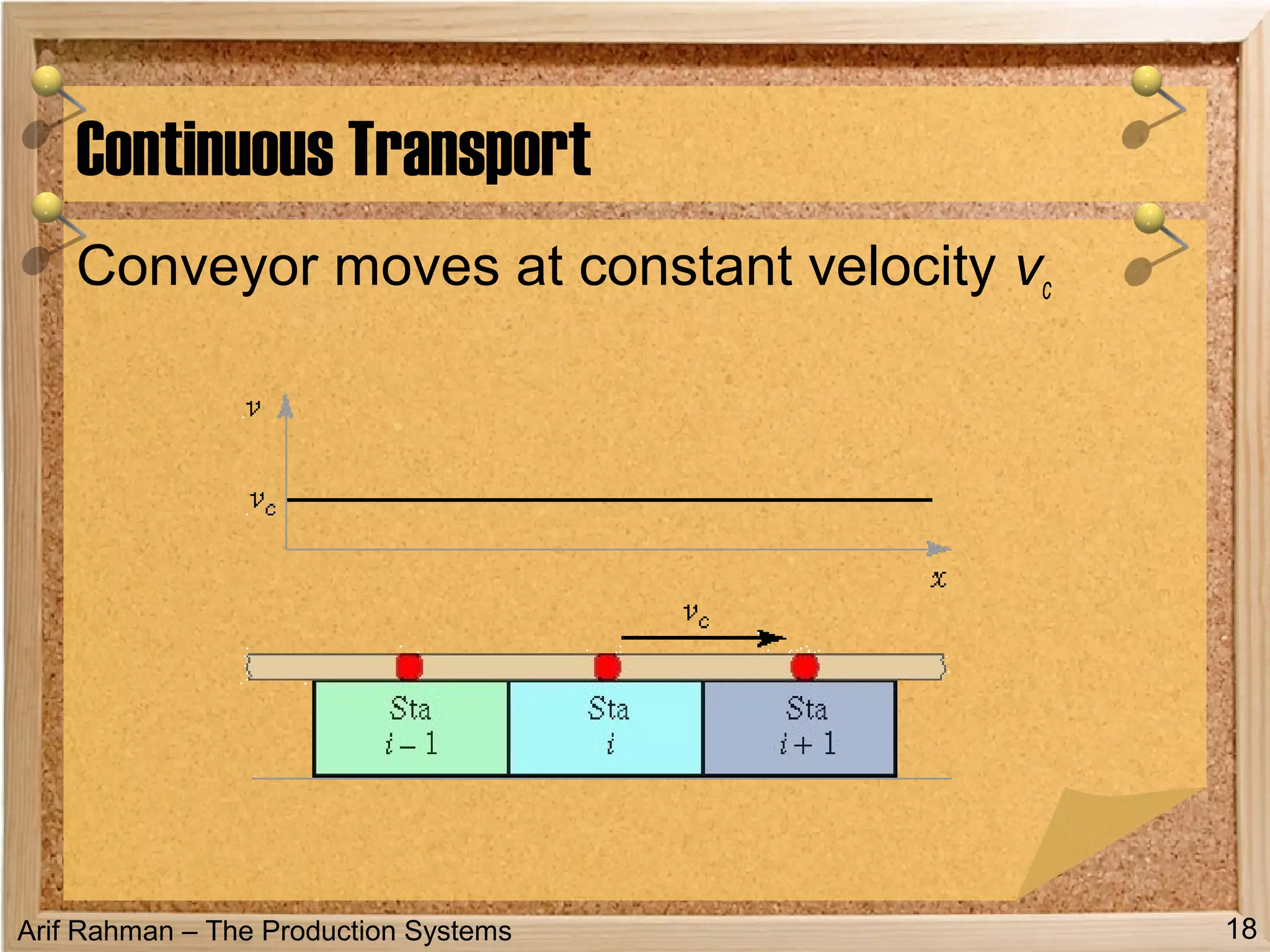


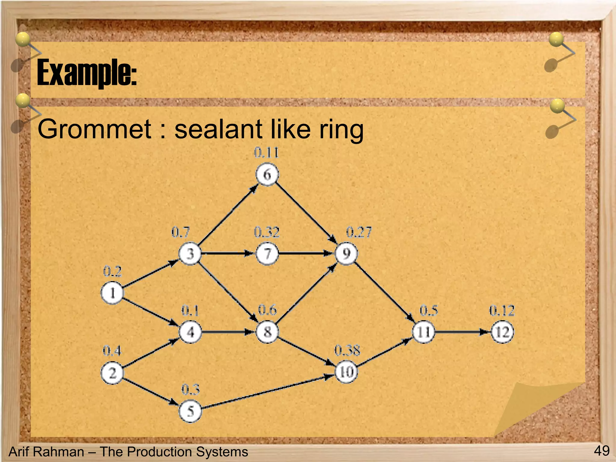

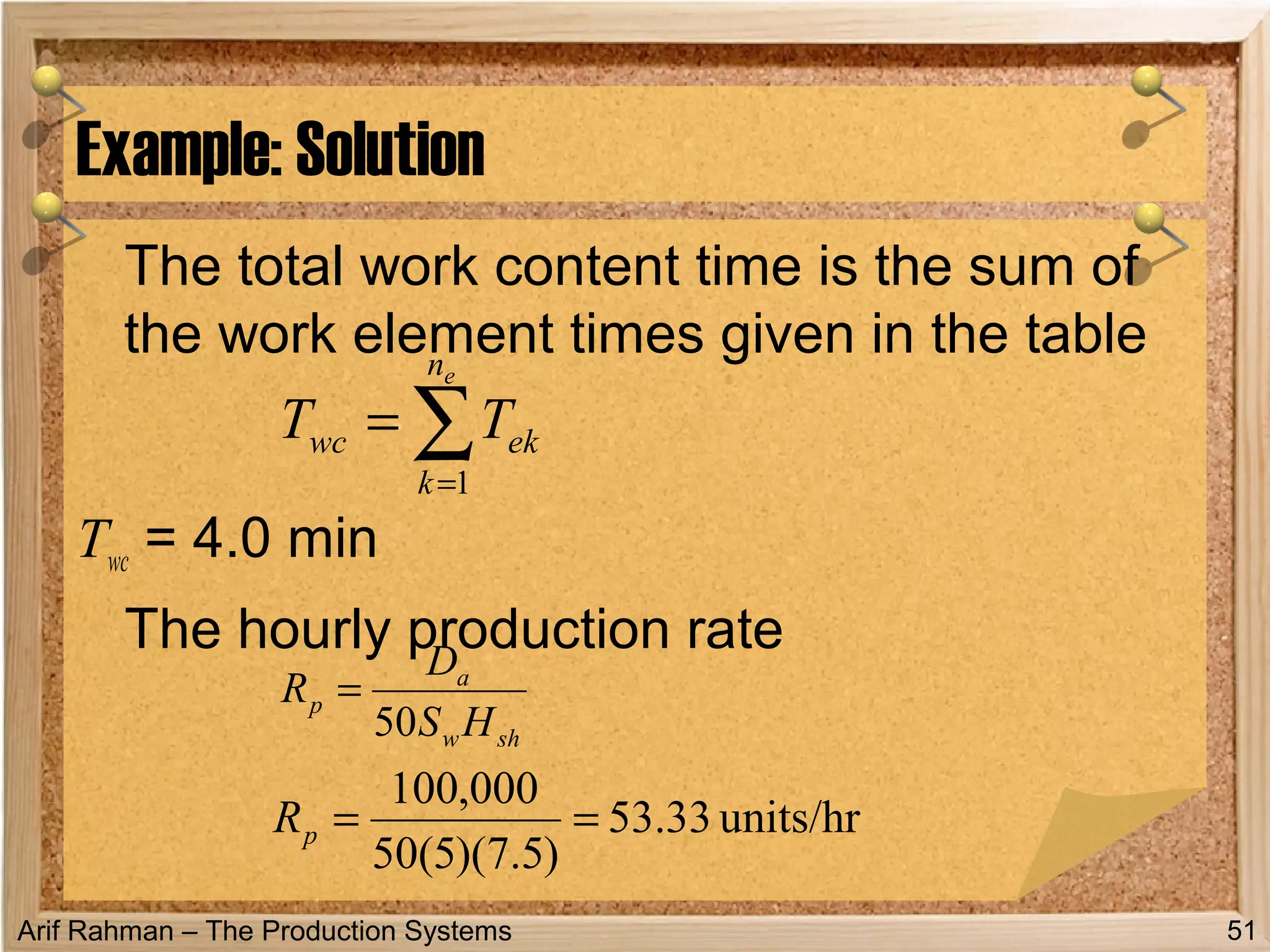


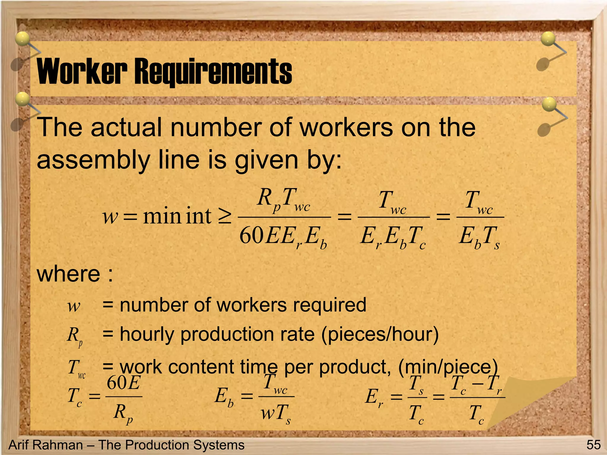
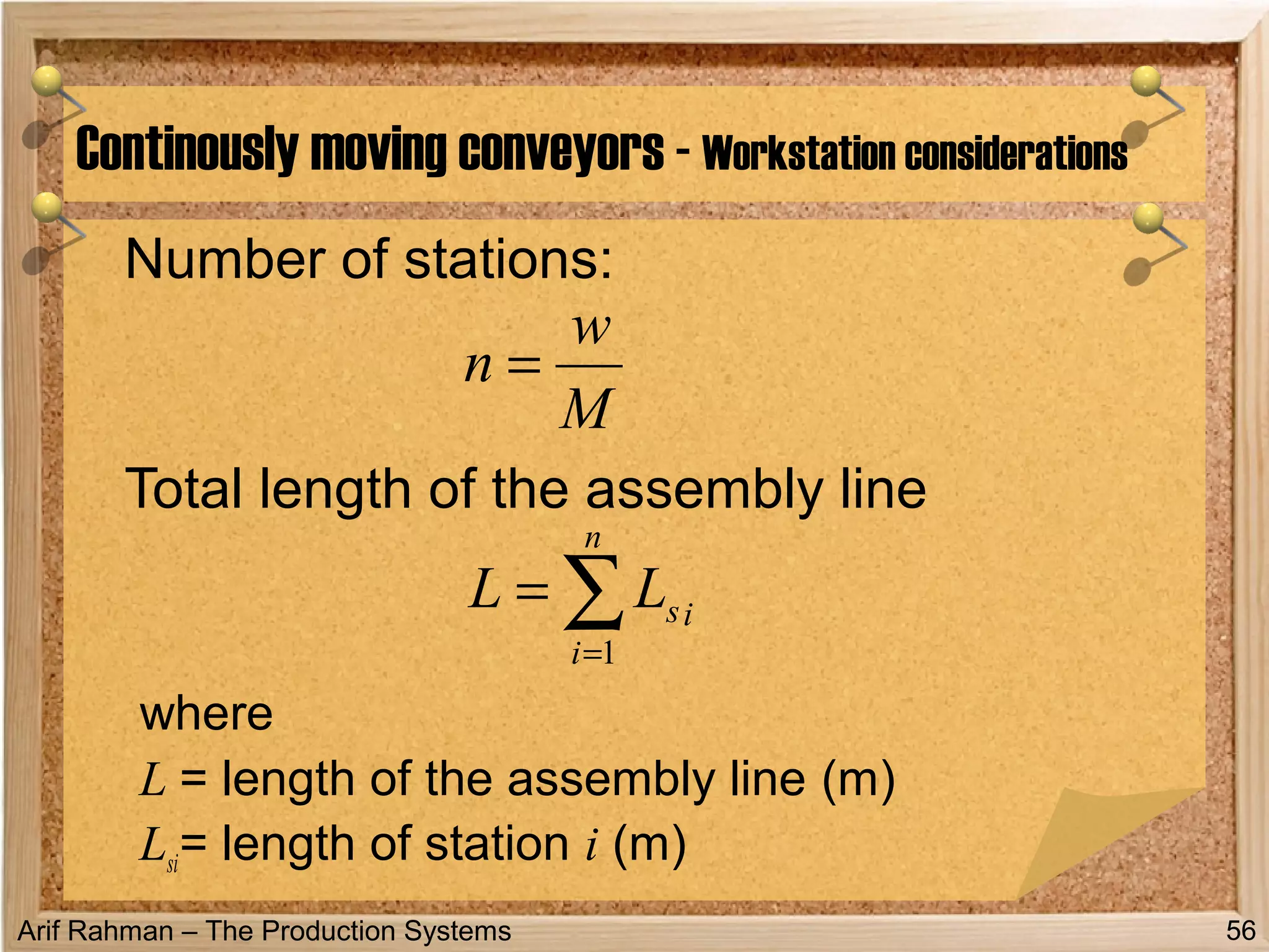


This document discusses manual assembly lines. It defines a manual assembly line as a production line consisting of a sequence of workstations where assembly tasks are performed by human workers as the product moves along the line. It notes that manual assembly lines are commonly used for high or medium demand products that require identical or similar assembly of standardized parts. The document outlines factors like specialization of labor, interchangeable parts, workflow principles, and line pacing that contribute to the productivity of manual assembly lines. It provides examples of typical products assembled on such lines and describes components like workstations, material handling, and different types of line pacing.