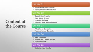
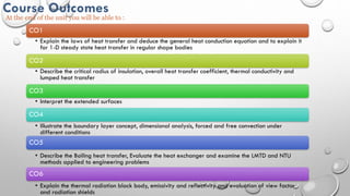
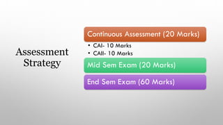
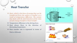
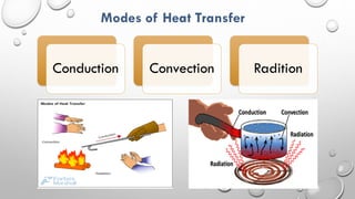
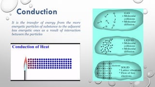
SlideShare a Scribd company logo
1 of 98
Download to read offline
A Course on
HEAT TRANSFER
Content of
the Course
Unit No. 01
• Introduction to Heat Transfer
• Steady State Heat Conduction
Unit No. 02
• Overall Heat Transfer
• Heat Source System
• Extended Surfaces
• Unsteady state heat Conduction
Unit No. 03
• Principles of Convection
• Free and Forced Convection
Unit No. 04
• Heat Exchanger
• Parallel and Counter flow HE
• TEMA Standards
Unit No. 05
• Radiation Heat Transfer
Prof. G. P. Badarkhe
Course Outcomes
At the end of the unit you will be able to :
CO1
• Explain the laws of heat transfer and deduce the general heat conduction equation and to explain it
for 1-D steady state heat transfer in regular shape bodies
CO2
• Describe the critical radius of insulation, overall heat transfer coefficient, thermal conductivity and
lumped heat transfer
CO3
• Interpret the extended surfaces
CO4
• Illustrate the boundary layer concept, dimensional analysis, forced and free convection under
different conditions
CO5
• Describe the Boiling heat transfer, Evaluate the heat exchanger and examine the LMTD and NTU
methods applied to engineering problems
CO6
• Explain the thermal radiation black body, emissivity and reflectivity and evaluation of view factor
and radiation shields
Assessment
Strategy
Continuous Assessment (20 Marks)
• CAI- 10 Marks
• CAII- 10 Marks
Mid Sem Exam (20 Marks)
End Sem Exam (60 Marks)
Books to Refer for Heat Transfer
1. S. P. Sukhatme, “A Textbook on Heat Transfer”, Tata McGraw Hill Publications,
3rd edition.
2. Y. A. Cengel, “Heat Transfer A Practical Approach”, Tata McGraw Hill Publication
s,3rd edition, 2006.
3. F. P. Incoropera, D. P. Dewitt, “Fundamentals of Heat and Mass Transfer”, John-
Wiley, 5th edition, 1990.
4. J. P. Holman, “Heat Transfer”, Tata McGraw Hill Publications, 9th edition, 2004.
5. R. K. Rajput, “Heat and Mass Transfer”
Pre-Requisites for Heat transfer
Calculus
Fluid Mechanics
Thermodynamics
Approach towards the Course
Theoretical
Experimental
Computational
Macroscopic and Microscopic
Point of View
 Macro means Big or at Bulk
• Considers certain quantity of matter(Overall behaviour)
• Requires simple mathematical Formulae
• Properties of the system are average values
• Few properties are needed to describe the system
 Micro means Small or at Molecular level
• Concerned directly with the structure of matter
• Analysis requires statistical method as the number of molecules are
very large
• Properties can not be easily measured by instruments
• Large number of variables are needed to describe the system
Difference Between Heat and Temperature
 HEAT
 Heat is energy in transit.
 Heat flows from hot body to cold body
 Temperature diff. is the driving force
 Usually denoted by Q
 Unit is joules or calorie
 TEMPERATURE
 Temperature is a measure of the amount of
energy possessed by the molecules of a
substance.
 Degree of Hotness
 can be used to predict the direction of heat
transfer
 Usually denoted by T
 Unit is degree Celsius or Kelvin
Heat Transfer
 Heat, which is the form of energy that can be
transferred from one system to another as a
result of temperature difference. The science
that deals with the determination of the rates
of such energy transfers is heat transfer.
 Temperature difference is the driving force.
 Heat always flows in the direction of
decreasing temperature.
 Heat transfer rate is expressed in terms of
Watt or Kilowatt.
Difference Between Thermodynamics and Heat
Transfer
Thermodynamics tells us:
•How much heat is transferred
How much work is done
Final state of the system
Heat transfer tells us:
How (with what modes) Q is transferred
At what rate Q is transferred
Temperature distribution inside the body
Example: Hot steel bar placed in a cold water bath
Applications of Heat Transfer
 Energy production and conversion
Steam Power plant, Solar energy conversion etc.
 Refrigeration and air conditioning
 Domestic applications
Ovens, Stoves, Toaster
 Cooling of electronic equipment
 Manufacturing / materials processing
Welding, Casting, Soldering, Laser machining
 Automobiles / aircraft design
 Nature (weather, climate etc)
 Chemical Industries
 Human Body
Applications of Heat Transfer Contd..
Rating and Sizing type of Problem
 Rating type of problem deal with the determination of heat transfer
rate for an existing system at a specified temperature difference.
 Sizing type of problem deal with the determination of the size of a
system in order to transfer heat at a specified rate for a specified
temperature difference.
Outcome of Unit No. 01
At the end of the unit you will be able to :
• Explain the laws of heat transfer and deduce the general heat
conduction equation and explain it for 1-D steady state heat transfer
in regular shape bodies
• Identify different modes of heat transfer in engineering applications
Modes of Heat Transfer
Conduction Convection Radition
Conduction
It is the transfer of energy from the more
energetic particles of substance to the adjacent
less energetic ones as a result of interaction
between the particles
Convection
Mode of energy transfer between a
solid surface and the adjacent fluid
that is in motion and it involves the
combined effect of conduction and
fluid motion
In the absence of any bulk fluid
motion, heat transfer between the solid
surface and adjacent fluid is by pure
conduction
Types of Convection
Natural Convection
Fluid motion occurs due to density variation
caused by temperature difference
Forced Convection
Fluid motion caused by
external agency
Practical Examples of Natural and Forced Convection
• Liquids gets converted
into vapours
Boiling
• Vapours gets converted
into liquids
Condensation
Radiation
Energy transfer in the form of electromagnetic waves because of
vibrational rotational motion of molecules and atoms which makes up
the matter or substance
• All physical matter emits thermal radiation at a particular level of temperature
• It does not require medium for the energy transfer to occur
Examples of radiation mode of heat transfer
Combined example of all modes of
heat transfer
Laws of Heat Transfer
Fundamental Laws
• Law of conservation of mass
Mass of a closed system is constant in the absence of nuclear reaction
For a control volume : Mass entering –Mass leaving = increase of mass
• Newton’s law of motion
Rate of change of momentum is directly proportional to applied force
𝑭 =
𝒅
𝒅𝒕
(𝒎𝑽)
• First law of thermodynamics
Principle of conservation of energy
dE = dQ - dW
Subsidiary Laws
• Fourier’s law of Heat Conduction
• Newton’s law of Cooling
• Laws of thermal radiation
Fourier’slaw of Heat Conduction
𝑸 ∝ ∆𝑻 𝑸 ∝
𝟏
∆𝒙
𝑸 ∝ 𝑨
𝑹𝒂𝒕𝒆 𝒐𝒇 𝑯𝒆𝒂𝒕 𝑪𝒐𝒏𝒅𝒖𝒄𝒕𝒊𝒐𝒏 ∝
𝑨𝒓𝒆𝒂)(𝑻𝒆𝒎𝒑𝒆𝒓𝒂𝒕𝒖𝒓𝒆 𝑫𝒊𝒇𝒇𝒆𝒓𝒆𝒏𝒄𝒆
𝑻𝒉𝒊𝒄𝒌𝒏𝒆𝒔𝒔
Fourier’s law of heat conduction states that rate of heat flow
through a simple homogeneous solids is directly
proportional to the area which is normal to the direction of
heat flow and the change in temperature with respect to the
length of the path of the heat flow
𝑸 ∝
𝑨 ∗ 𝒅𝑻
𝐝𝒙
𝑸
𝑨
= 𝒒 ∝
𝐝𝑻
𝐝𝒙
𝒒 = − 𝒌
𝐝𝑻
𝐝𝒙
Where q is heat flux
- Sign indicates heat flow in the direction of decreasing temp.
ThermalConductivity
Ability of a material to conduct heat
Rate of heat transfer through a unit thickness of the material
per unit area per unit temperature difference
𝒌 =
𝑸 ∗ 𝒅𝒙
𝑨 ∗ 𝒅𝑻
Unit of thermal conductivity : 𝑾
𝒎𝒌
𝒐𝒓 𝑾
𝒎℃
For Example Copper has Thermal Conductivity of 401 𝐖
𝐦𝐤
Thermal Conductivity depend on
 Material Structure
 Density of Material
 Moisture Content
 Temperature
Insulator
Conductor
Effect of Alloying:
k(Copper)= 401 W/m.K
K(Nickel)=91 W/m.K
K(constantan: 55% Cu & 45% Ni)= 23 w/m.K
Effect of Temperature:
K(Metals) α 1/T
Aluminium and Uranium as exception
(Mercury)
K(Non Metals) α T
K(Gases) α T
K(Liquids) α 1/T
Water as exception
Determination of Thermal
Conductivity
Heat Capacity and Thermal Diffusivity
Specific Heat Cp: J/kg.K
Cp(water)=4.18 kJ/kg K
Cp(iron)=0.45 kJ/kg K
Cp is the capacity to store thermal
energy
k(water)=0.608 W/m K
k(iron)=80.2 W/m K
k is the capacity to conduct thermal
energy
Heat Capacity 𝝆𝑪𝒑 : J/cubic m. k
Thermal Diffusivity
∝=
𝐻𝑒𝑎𝑡 𝐶𝑜𝑛𝑑𝑢𝑐𝑡𝑖𝑜𝑛
𝐻𝑒𝑎𝑡 𝑆𝑡𝑜𝑟𝑎𝑔𝑒
=
𝑘
𝜌𝐶𝑝
Unit of ∝ : Sq. m /Sec
Newtons Law of Cooling
Rate of heat transfer is directly proportional
to the temperature difference between
surface & surrounding and area which is in
contact.
𝑄𝐶𝑜𝑛𝑣. = ℎ 𝐴𝑠 𝑇𝑠 − 𝑇∞
𝑄𝐶𝑜𝑛𝑣. ∝ 𝐴𝑠 𝑇𝑠 − 𝑇∞
 𝑯𝒆𝒂𝒕 𝑻𝒓𝒂𝒏𝒔𝒇𝒆𝒓 𝑪𝒐𝒆𝒇𝒇𝒊𝒄𝒊𝒆𝒏𝒕:
ℎ =
𝑄𝐶𝑜𝑛𝑣.
𝐴𝑠 𝑇𝑠− 𝑇∞
= 𝑊
𝑚2𝑘 𝑜𝑟 ℃
 Whose value depends upon:
 Surface Geometry
 Nature of Fluid Motion
 Properties of Fluid
 Bulk Fluid Velocity
Stefan-Boltzmann's Law
It sates that emissive power of a black body is directly
proportional to fourth power of its absolute temperature.
𝑄
𝐴
= 𝐸𝑏𝑙𝑎𝑐𝑘 ∝ 𝑇4
𝐸𝑏𝑙𝑎𝑐𝑘 = 𝜎 𝑇
4
or𝑄𝐵𝑙𝑎𝑐𝑘 𝑜𝑟 𝑚𝑎𝑥= 𝜎𝐴𝑠 𝑇𝑠
4
Where 𝜎 is Stefan-Boltzmann constant and
has the value of 5.67 ∗ 10−8 𝑊
𝑚2𝑘4
 For Real Surfaces:
𝑄𝑅𝑒𝑎𝑙 = 𝜀𝐴𝑠 𝜎 𝑇𝑠
4
Co-ordinate systems
Generalised Heat Conduction equation in
Cartesian Co-ordinate systems
Consider a infinitesimal small elemental volume of side dx, dy & dz as
shown in figure in a medium in which temperature is varying with
location and time
Let kx ky kz be the thermal conductivities in x, y, and z direction
respectively
Energy balance equation for volumetric element (control volume) is given by:
𝑁𝑒𝑡 ℎ𝑒𝑎𝑡 𝑎𝑐𝑐𝑢𝑚𝑢𝑙𝑎𝑡𝑒𝑑 𝑖𝑛 𝑡ℎ𝑒 𝑒𝑙𝑒𝑚𝑒𝑛𝑡 𝑑𝑢𝑒 𝑡𝑜 𝑐𝑜𝑛𝑑𝑢𝑐𝑡𝑖𝑜𝑛 𝑜𝑓 ℎ𝑒𝑎𝑡 𝑓𝑟𝑜𝑚 𝑎𝑙𝑙 𝑡ℎ𝑒
𝑑𝑖𝑟𝑒𝑐𝑡𝑖𝑜𝑛 𝑐𝑜𝑛𝑠𝑖𝑑𝑒𝑟𝑒𝑑(𝐴) + ℎ𝑒𝑎𝑡 𝑔𝑒𝑛𝑒𝑟𝑎𝑡𝑒𝑑 𝑤𝑖𝑡ℎ𝑖𝑛 𝑡ℎ𝑒 𝑒𝑙𝑒𝑚𝑒𝑛𝑡(𝐵) =
𝑅𝑎𝑡𝑒 𝑜𝑓 𝑐ℎ𝑎𝑛𝑔𝑒 𝑜𝑓𝑒𝑛𝑒𝑟𝑦 𝑐𝑜𝑛𝑡𝑒𝑛𝑡 𝑜𝑓 𝑡ℎ𝑒 𝑒𝑙𝑒𝑚𝑒𝑛𝑡(C)………………………………..(1)
A. Net heat accumulated in the element due to conduction of heat from all the
direction considered
Quantity of heat entering the element in x direction per unit time i.e. Heat
influx
𝑄𝑥 = − 𝑘𝑥. 𝐴.
𝜕𝑇
𝜕𝑥
𝑄𝑥 = − 𝑘𝑥. 𝑑𝑦. 𝑑𝑧 .
𝜕𝑇
𝜕𝑥
Quantity of heat leaving the element in x direction per unit time i.e.
Heat efflux
𝑄𝑥+𝑑𝑥 = 𝑄𝑥 +
𝜕
𝜕𝑥
𝑄𝑥 𝑑𝑥
Heat accumulated in the element due to heat flow in x direction
per unit time
𝑑𝑄𝑥 = 𝑄𝑥 − 𝑄𝑥 +
𝜕
𝜕𝑥
𝑄𝑥 𝑑𝑥
𝑑𝑄𝑥 = −
𝜕
𝜕𝑥
𝑄𝑥 𝑑𝑥
𝑑𝑄𝑥 = −
𝜕
𝜕𝑥
− 𝑘𝑥 𝑑𝑦. 𝑑𝑧
𝜕𝑇
𝜕𝑥
𝑑𝑥
𝑑𝑄𝑥 =
𝜕
𝜕𝑥
𝑘𝑥
𝜕𝑇
𝜕𝑥
𝑑𝑥. 𝑑𝑦. 𝑑𝑧
Similarly heat accumulated due to heat flow by conduction along y
and z direction will be:
𝑑𝑄𝑦 =
𝜕
𝜕𝑦
𝑘𝑦
𝜕𝑇
𝜕𝑦
𝑑𝑥. 𝑑𝑦. 𝑑𝑧
𝑑𝑄𝑧 =
𝜕
𝜕𝑧
𝑘𝑧
𝜕𝑇
𝜕𝑧
𝑑𝑥. 𝑑𝑦. 𝑑𝑧
Net heat accumulated in the element due to conduction of heat from all
the direction considered per unit time =
𝜕
𝜕𝑥
𝑘𝑥
𝜕𝑇
𝜕𝑥
+
𝜕
𝜕𝑦
𝑘𝑦
𝜕𝑇
𝜕𝑦
+
𝜕
𝜕𝑧
𝑘𝑧
𝜕𝑇
𝜕𝑧
𝑑𝑥. 𝑑𝑦. 𝑑𝑧
--------------------(i)
B. Total Heat generated within the element per unit time
𝑄𝑔 = 𝑞𝑔
′′′ ∗ 𝑑𝑥. 𝑑𝑦. 𝑑𝑧
--------------- (ii)
C. Rate of change of energy content of the element
𝑚. 𝐶𝑝.
𝜕𝑇
𝜕𝜏
𝜌. 𝑉. 𝐶𝑝 .
𝜕𝑇
𝜕𝜏
𝜌. 𝐶𝑝.
𝜕𝑇
𝜕𝜏
. 𝑑𝑥. 𝑑𝑦. 𝑑𝑧
------------------(iii)
Putting value of (i), (ii),(iii) in equation no. (1) the heat balance equation
will be
𝝏
𝝏𝒙
𝒌𝒙
𝝏𝑻
𝝏𝒙
+
𝝏
𝝏𝒚
𝒌𝒚
𝝏𝑻
𝝏𝒚
+
𝝏
𝝏𝒛
𝒌𝒛
𝝏𝑻
𝝏𝒛
𝒅𝒙. 𝒅𝒚. 𝒅𝒛 + 𝒒𝒈
′′′
∗ 𝒅𝒙. 𝒅𝒚. 𝒅𝒛 = 𝛒. 𝑪𝒑.
𝝏𝑻
𝝏𝝉
. 𝐝𝐱. 𝐝𝐲. 𝐝𝐳
𝝏
𝝏𝒙
𝒌𝒙
𝝏𝑻
𝝏𝒙
+
𝝏
𝝏𝒚
𝒌𝒚
𝝏𝑻
𝝏𝒚
+
𝝏
𝝏𝒛
𝒌𝒛
𝝏𝑻
𝝏𝒛
+ 𝒒𝒈
′′′
= 𝛒. 𝑪𝒑.
𝝏𝑻
𝝏𝝉
This is known as generalised heat conduction equation in cartesian co-ordinate
system
If material or medium is Isotropic then kx=ky=kz=k then
above equation becomes
𝑘
𝜕
𝜕𝑥
𝜕𝑇
𝜕𝑥
+
𝜕
𝜕𝑦
𝜕𝑇
𝜕𝑦
+
𝜕
𝜕𝑧
𝜕𝑇
𝜕𝑧
+ 𝑞𝑔
′′′ = 𝜌. 𝐶𝑝.
𝜕𝑇
𝜕𝜏
𝝏𝟐
𝑻
𝝏𝒙𝟐 +
𝝏𝟐
𝑻
𝝏𝒚𝟐 +
𝝏𝟐
𝑻
𝝏𝒛𝟐 +
𝒒𝒈
′′′
𝒌
=
𝝆. 𝑪𝒑
𝒌
.
𝝏𝑻
𝝏𝝉
𝝏𝟐𝑻
𝝏𝒙𝟐
+
𝝏𝟐𝑻
𝝏𝒚𝟐
+
𝝏𝟐𝑻
𝝏𝒛𝟐
+
𝒒𝒈
′′′
𝒌
=
𝟏
𝜶
.
𝝏𝑻
𝝏𝝉
𝜶=
𝒌
𝝆.𝑪𝒑
Thermal diffusivity
Simplified forms of heat conduction equation in cartesian
coordinate system
 Unsteady state heat flow with no internal heat generation
(Fourier’s Equation)
𝝏𝟐𝑻
𝝏𝒙𝟐
+
𝝏𝟐𝑻
𝝏𝒚𝟐
+
𝝏𝟐𝑻
𝝏𝒛𝟐
=
𝟏
𝜶
.
𝝏𝑻
𝝏𝝉
 Steady state heat flow with heat generation(Poisson’s equation)
𝝏𝟐𝑻
𝝏𝒙𝟐 +
𝝏𝟐𝑻
𝝏𝒚𝟐 +
𝝏𝟐𝑻
𝝏𝒛𝟐 +
𝒒𝒈
′′′
𝒌
= 𝟎
 Steady state heat flow without internal heat generation(Laplace
Equation)
𝝏𝟐𝑻
𝝏𝒙𝟐
+
𝝏𝟐𝑻
𝝏𝒚𝟐
+
𝝏𝟐𝑻
𝝏𝒛𝟐
= 𝟎
 Steady state, one dimensional heat flow with heat generation
𝝏𝟐
𝑻
𝝏𝒙𝟐
+
𝒒𝒈
′′′
𝒌
= 𝟎
 Steady state, one dimensional heat flow without heat generation
𝝏𝟐
𝑻
𝝏𝒙𝟐
= 𝟎
 Unsteady state, one dimensional heat flow without heat
Generation
𝝏𝟐𝑻
𝝏𝒙𝟐 =
𝟏
𝜶
.
𝝏𝑻
𝝏𝝉
Generalised Heat Conduction equation in
Polar/Cylindrical Co-ordinate systems
Consider a infinitesimally small elemental volume having the
coordinates r,𝝓 & z as shown in figure in a medium in which
temperature is varying with location and time
Let us assume that Thermal Conductivity k, Density 𝛒 and
specific heat Cp do not change with space
Volume of the element rd𝝓.dr.dz
Energy balance equation for volumetric element (control volume)
is given by:
𝐍𝐞𝐭 𝐡𝐞𝐚𝐭 𝐚𝐜𝐜𝐮𝐦𝐮𝐥𝐚𝐭𝐞𝐝 𝐢𝐧 𝐭𝐡𝐞 𝐞𝐥𝐞𝐦𝐞𝐧𝐭 𝐝𝐮𝐞 𝐭𝐨 𝐜𝐨𝐧𝐝𝐮𝐜𝐭𝐢𝐨𝐧 𝐨𝐟 𝐡𝐞𝐚𝐭 𝐟𝐫𝐨𝐦 𝐚𝐥𝐥 𝐭𝐡𝐞
𝐝𝐢𝐫𝐞𝐜𝐭𝐢𝐨𝐧 𝐜𝐨𝐧𝐬𝐢𝐝𝐞𝐫𝐞𝐝(𝐀) + 𝐡𝐞𝐚𝐭 𝐠𝐞𝐧𝐞𝐫𝐚𝐭𝐞𝐝 𝐰𝐢𝐭𝐡𝐢𝐧 𝐭𝐡𝐞 𝐞𝐥𝐞𝐦𝐞𝐧𝐭(𝐁) =
𝐑𝐚𝐭𝐞 𝐨𝐟 𝐜𝐡𝐚𝐧𝐠𝐞 𝐨𝐟𝐞𝐧𝐞𝐫𝐲 𝐜𝐨𝐧𝐭𝐞𝐧𝐭 𝐨𝐟 𝐭𝐡𝐞 𝐞𝐥𝐞𝐦𝐞𝐧𝐭 (C)………………………………..(1
)
Net heat accumulated in the
element due to conduction of
heat from all the direction
considered
Heat Generated within
the element
Rate of change of
energy content of the
element
+ =
A. Net heat accumulated in the element due to conduction of heat
from all the direction considered
Heat Flow in Radial Direction
Quantity of heat entering the element in r direction (z- 𝝓 plane) per
unit time i.e. Heat influx in r direction
𝑸𝒓 = −𝒌. 𝑨.
𝝏𝑻
𝝏𝒓
𝑸𝒓 = −𝒌. 𝒓𝒅𝝓. 𝒅𝒛 .
𝝏𝑻
𝝏𝒓
Quantity of heat leaving the element in r direction per unit time i.e.
Heat efflux
𝐐𝐫+𝐝𝒓 = 𝐐𝒓 +
𝛛
𝛛𝒓
𝐐𝒓 𝐝𝐫
Net Heat accumulated in the element due to heat flow in radial
direction per unit time
𝐝𝐐𝒓 = 𝐐𝒓 − 𝐐𝒓 +
𝛛
𝛛𝒓
𝐐𝒓 𝐝𝒓
𝐝𝐐𝒓 = −
𝛛
𝛛𝒓
𝐐𝒓 𝐝𝐫
𝒅𝑸𝒓 = −
𝝏
𝝏𝒓
− 𝒌 𝒓𝒅𝝓. 𝒅𝒛
𝝏𝑻
𝝏𝒓
𝒅𝒓
𝒅𝑸𝒓 = 𝒌 𝒅𝒓. 𝒅𝝓. 𝒅𝒛
𝝏
𝝏𝒓
𝒓
𝝏𝑻
𝝏𝒓
𝒅𝑸𝒓 = 𝒌(𝒅𝒓. 𝒅𝝓. 𝒅𝒛) 𝒓
𝝏𝟐𝑻
𝝏𝒓𝟐
+
𝝏𝑻
𝝏𝒓
𝒅𝑸𝒓 = 𝒌(𝒅𝒓. 𝒓𝒅𝝓. 𝒅𝒛)
𝝏𝟐𝑻
𝝏𝒓𝟐
+
𝟏
𝒓
𝝏𝑻
𝝏𝒓
Heat Flow in Tangential i.e. 𝝓 (r-z plane) Direction
Quantity of heat entering the element in 𝝓 direction (r-z plane)
per unit time i.e. Heat influx in 𝝓 direction
𝑸𝝓 = −𝒌. 𝑨.
𝝏𝑻
𝒓. 𝝏𝝓
𝑸𝝓 = −𝒌. 𝒅𝒓. 𝒅𝒛 .
𝝏𝑻
𝒓. 𝝏𝝓
Quantity of heat leaving the element in 𝝓 direction per unit time i.e.
Heat efflux
𝐐𝝓+𝐝𝝓 = 𝐐𝝓 +
𝛛
𝒓. 𝛛𝝓
𝐐𝝓 𝒓𝐝𝝓
Net Heat accumulated in the element due to heat flow in tangential
direction per unit time
𝐝𝐐𝝓 = 𝐐𝝓 − 𝐐𝝓+𝒅𝝓
Net Heat accumulated in the element due to heat flow in
tangential direction per unit time
𝐝𝐐𝝓 = 𝐐𝝓 − 𝐐𝝓 +
𝛛
𝒓. 𝛛𝝓
𝐐𝝓 𝒓𝐝𝝓
𝐝𝐐𝝓 = −
𝛛
𝒓. 𝛛𝝓
𝐐𝝓 𝒓𝐝𝝓
𝒅𝑸𝝓 = −
𝝏
𝒓. 𝛛𝝓
− 𝒌 𝒅𝒓. 𝒅𝒛
𝝏𝑻
𝒓. 𝛛𝝓
𝒓𝐝𝝓
𝒅𝑸𝝓 = 𝒌 𝒅𝒓. 𝒅𝝓. 𝒅𝒛
𝝏
𝝏𝝓
𝟏
𝒓
𝝏𝑻
𝝏𝝓
𝒅𝑸𝝓 = 𝒌 𝒅𝒓. 𝒓𝒅𝝓. 𝒅𝒛
𝟏
𝒓𝟐
𝝏
𝝏𝝓
𝝏𝑻
𝝏𝝓
𝒅𝑸𝝓 = 𝒌 𝒅𝒓. 𝒓𝒅𝝓. 𝒅𝒛
𝟏
𝒓𝟐
𝝏𝟐
𝑻
𝝏𝝓𝟐
Heat Flow in Axial i.e. z (r- 𝝓 plane) Direction
Quantity of heat entering the element in z direction (r- 𝛟 plane)
per unit time i.e. Heat influx in 𝒛 direction
𝑸𝒛 = −𝒌. 𝑨.
𝝏𝑻
𝝏𝒛
𝑸𝒛 = −𝒌. 𝒓𝒅𝝓. 𝒅𝒓 .
𝝏𝑻
𝝏𝒛
Heat accumulated in the element due to heat flow in axial
direction per unit time
𝐝𝐐𝒛 = 𝐐𝒛 − 𝐐𝒛 +
𝛛
𝛛𝒛
𝐐𝒛 𝐝𝒛
𝐝𝐐𝒛 = −
𝛛
𝛛𝒛
𝐐𝒛 𝐝𝐳
Quantity of heat leaving the element in r direction per unit time i.e.
Heat efflux
𝐐𝐳 = 𝐐𝒛 +
𝛛
𝛛𝒛
𝐐𝒛 𝐝𝐳
𝐝𝐐𝐳 = −
𝛛
𝛛𝐳
− 𝐤 𝐫𝐝𝛟. 𝐝𝐫
𝛛𝐓
𝛛𝐳
𝐝𝐳
𝐝𝐐𝐳 = 𝐤(𝐝𝐫. 𝐫𝐝𝛟. 𝐝𝐳)
𝛛𝟐
𝐓
𝛛𝐳𝟐
Net heat accumulated in the element due to conduction of
heat from all the direction considered per unit time =
𝝏𝟐𝑻
𝝏𝒓𝟐
+
𝟏
𝒓
𝝏𝑻
𝝏𝒓
+
𝟏
𝒓𝟐
𝝏𝟐𝑻
𝝏𝝓𝟐
+
𝛛𝟐𝐓
𝛛𝐳𝟐
𝐤(𝐝𝐫. 𝐫𝐝𝛟. 𝐝𝐳)
--------------------(i)
B. Total Heat generated within the element per unit time
𝑸𝒈 = 𝒒𝒈
′′′ ∗ 𝐝𝐫. 𝐫𝐝𝛟. 𝐝𝐳
--------------- (ii)
C. Rate of change of energy content of the element
𝐦. 𝐂𝐩.
𝛛𝐓
𝛛𝛕
𝛒. 𝐕. 𝐂𝐩 .
𝛛𝐓
𝛛𝛕
𝛒. 𝐂𝐩.
𝛛𝐓
𝛛𝛕
. 𝐝𝐫. 𝐫𝐝𝛟. 𝐝𝐳
------------------(iii)
Now
A + B = C
Net heat accumulated in the
element due to conduction of
heat from all the direction
considered
Heat Generated within
the element
Rate of change of
energy content of the
element
𝝏𝟐
𝑻
𝝏𝒓𝟐
+
𝟏
𝒓
𝝏𝑻
𝝏𝒓
+
𝟏
𝒓𝟐
𝝏𝟐
𝑻
𝝏𝝓𝟐
+
𝝏𝟐
𝑻
𝛛𝒛𝟐
𝐤(𝐝𝐫. 𝐫𝐝𝛟. 𝐝𝐳)
𝒒𝒈
′′′ ∗ 𝐝𝐫. 𝐫𝐝𝛟. 𝐝𝐳
𝛒. 𝑪𝒑.
𝝏𝑻
𝝏𝝉
. 𝐝𝐫. 𝐫𝐝𝛟. 𝐝𝐳
+
=
𝝏𝟐𝑻
𝝏𝒓𝟐
+
𝟏
𝒓
𝝏𝑻
𝝏𝒓
+
𝟏
𝒓𝟐
𝝏𝟐𝑻
𝝏𝝓𝟐
+
𝛛𝟐𝐓
𝛛𝐳𝟐
𝐤 𝐝𝐫. 𝐫𝐝𝛟. 𝐝𝐳 + 𝒒𝒈
′′′ ∗ 𝐝𝐫. 𝐫𝐝𝛟. 𝐝𝐳
= 𝛒. 𝐂𝐩.
𝛛𝐓
𝛛𝛕
. 𝐝𝐫. 𝐫𝐝𝛟. 𝐝𝐳
Dividing both side by 𝑑𝑟. 𝑟𝑑𝜙. 𝑑𝑧
𝝏𝟐
𝑻
𝝏𝒓𝟐
+
𝟏
𝒓
𝝏𝑻
𝝏𝒓
+
𝟏
𝒓𝟐
𝝏𝟐
𝑻
𝝏𝝓𝟐
+
𝝏𝟐
𝑻
𝝏𝒛𝟐
𝒌 + 𝒒𝒈
′′′
= 𝝆. 𝑪𝒑.
𝝏𝑻
𝝏𝝉
Or
𝝏𝟐𝑻
𝝏𝒓𝟐
+
𝟏
𝒓
𝝏𝑻
𝝏𝒓
+
𝟏
𝒓𝟐
𝝏𝟐𝑻
𝝏𝝓𝟐
+
𝝏𝟐𝑻
𝝏𝒛𝟐
+
𝒒𝒈
′′′
𝒌
=
𝝆. 𝑪𝒑
𝒌
.
𝝏𝑻
𝝏𝝉
𝝏𝟐𝑻
𝝏𝒓𝟐
+
𝟏
𝒓
𝝏𝑻
𝝏𝒓
+
𝟏
𝒓𝟐
𝝏𝟐𝑻
𝝏𝝓𝟐
+
𝝏𝟐𝑻
𝝏𝒛𝟐
+
𝒒𝒈
′′′
𝒌
=
𝟏
𝜶
.
𝝏𝑻
𝝏𝝉
For Steady state, without internal heat generation and one dimensional flow
𝝏𝟐𝑻
𝝏𝒓𝟐
+
𝟏
𝒓
𝝏𝑻
𝝏𝒓
= 𝟎
Generalised Heat Conduction equation in
Spherical Co-ordinate systems
Consider a infinitesimally small elemental volume having the coordinates r, 𝜙 & 𝜃 as
shown in figure in a medium in which temperature is varying with location and time
Let us assume that Thermal Conductivity k, Density 𝜌 and specific heat Cp
do not change with space
Volume of the element dr. rd𝜃. 𝑟𝑠𝑖𝑛 𝜃d𝜙
Energy balance equation for volumetric element (control volume) is given by:
𝑁𝑒𝑡 ℎ𝑒𝑎𝑡 𝑎𝑐𝑐𝑢𝑚𝑢𝑙𝑎𝑡𝑒𝑑 𝑖𝑛 𝑡ℎ𝑒 𝑒𝑙𝑒𝑚𝑒𝑛𝑡 𝑑𝑢𝑒 𝑡𝑜 𝑐𝑜𝑛𝑑𝑢𝑐𝑡𝑖𝑜𝑛 𝑜𝑓 ℎ𝑒𝑎𝑡 𝑓𝑟𝑜𝑚 𝑎𝑙𝑙 𝑡ℎ𝑒
𝑑𝑖𝑟𝑒𝑐𝑡𝑖𝑜𝑛 𝑐𝑜𝑛𝑠𝑖𝑑𝑒𝑟𝑒𝑑(𝐴) + ℎ𝑒𝑎𝑡 𝑔𝑒𝑛𝑒𝑟𝑎𝑡𝑒𝑑 𝑤𝑖𝑡ℎ𝑖𝑛 𝑡ℎ𝑒 𝑒𝑙𝑒𝑚𝑒𝑛𝑡(𝐵) =
𝑅𝑎𝑡𝑒 𝑜𝑓 𝑐ℎ𝑎𝑛𝑔𝑒 𝑜𝑓𝑒𝑛𝑒𝑟𝑦 𝑐𝑜𝑛𝑡𝑒𝑛𝑡 𝑜𝑓 𝑡ℎ𝑒 𝑒𝑙𝑒𝑚𝑒𝑛𝑡(C)………………………………..(1)
Net heat accumulated in the
element due to conduction of
heat from all the direction
considered
Heat Generated within
the element
Rate of change of
energy content of the
element
+ =
A. Net heat accumulated in the element due to conduction of heat from all the
direction considered
Heat Flow in Radial (r) Direction
Quantity of heat entering the element in r direction (𝜃 - 𝜙 plane) per unit time
i.e. Heat influx in r direction
𝑄𝑟 = −𝑘. 𝐴.
𝜕𝑇
𝜕𝑟
𝑄𝑟 = −𝑘. rd𝜃. 𝑟𝑠𝑖𝑛 𝜃𝑑𝜙 .
𝜕𝑇
𝜕𝑟
Quantity of heat leaving the element in r direction per
unit time i.e. Heat efflux
𝑄r+𝑑𝑟 = 𝑄𝑟 +
𝜕
𝜕𝑟
𝑄𝑟 𝑑r
Net Heat accumulated in the element due to heat flow in radial direction
per unit time
𝑑𝑄𝑟 = 𝑄𝑟 − 𝑄𝑟 +
𝜕
𝜕𝑟
𝑄𝑟 𝑑𝑟
𝑑𝑄𝑟 = −
𝜕
𝜕𝑟
𝑄𝑟 𝑑r
𝑑𝑄𝑟 = −
𝜕
𝜕𝑟
−𝑘 𝑟𝑑𝜃. 𝑟 sin 𝜃𝑑𝜙
𝜕𝑇
𝜕𝑟
𝑑𝑟
𝑑𝑄𝑟 = 𝑘 𝑑𝑟. 𝑑𝜃. sin 𝜃𝑑𝜙
𝜕
𝜕𝑟
𝑟2
𝜕𝑇
𝜕𝑟
𝑑𝑄𝑟 = 𝑘 𝑑𝑟. 𝑟𝑑𝜃. 𝑟sin 𝜃𝑑𝜙
1
𝑟2
𝜕
𝜕𝑟
𝑟2
𝜕𝑇
𝜕𝑟
Heat Flow in 𝜙 (r-𝜃 plane) Direction
Quantity of heat entering the element in 𝜙 direction (r-𝜃 plane) per unit
time i.e. Heat influx in 𝜙 direction
𝑄𝜙 = −𝑘. 𝐴.
𝜕𝑇
𝑟. sin 𝜃 𝜕𝜙
𝑄𝜙 = −𝑘. 𝑑𝑟. 𝑟𝑑𝜃 .
𝜕𝑇
𝑟. sin 𝜃 𝜕𝜙
Quantity of heat leaving the element in 𝜙 direction per
unit time i.e. Heat efflux
𝑄𝜙+𝑑𝜙 = 𝑄𝜙 +
𝜕
𝑟. sin 𝜃 𝜕𝜙
𝑄𝜙 𝑟. sin 𝜃 𝑑𝜙
Net Heat accumulated in the element due to heat flow in
𝜙 per unit time
𝑑𝑄𝜙 = 𝑄𝜙 − 𝑄𝜙+𝑑𝜙
Net Heat accumulated in the element due to heat flow in 𝜙 per unit time
𝑑𝑄𝜙 = 𝑄𝜙 − 𝑄𝜙 +
𝜕
𝑟 sin 𝜃 𝜕𝜙
𝑄𝜙 𝑟 sin 𝜃. 𝑑𝜙
𝑑𝑄𝜙 = −
𝜕
𝑟 sin 𝜃 𝜕𝜙
𝑄𝜙 𝑟 sin 𝜃. 𝑑𝜙
𝑑𝑄𝜙 = −
𝜕
𝑟 sin 𝜃 𝜕𝜙
− 𝑘 𝑑𝑟. 𝑟𝑑𝜃
𝜕𝑇
𝑟 sin 𝜃 𝜕𝜙
𝑟 sin 𝜃. 𝑑𝜙
𝑑𝑄𝜙 = 𝑘 𝑑𝑟. 𝑟𝑑𝜃. 𝑟sin 𝜃𝑑𝜙
1
𝑟2 sin2 𝜃
𝜕2
𝑇
𝜕𝜙2
Heat Flow in 𝜃(r-𝜙plane) Direction
Quantity of heat entering the element in 𝜃 direction (r-𝜙 plane) per unit
time i.e. Heat influx in 𝜃 direction
𝑄𝜃 = −𝑘. 𝐴.
𝜕𝑇
𝑟𝜕𝜃
𝑄𝜃 = −𝑘. 𝑑𝑟. 𝑟sin 𝜃𝑑𝜙 .
𝜕𝑇
𝑟𝜕𝜃
Quantity of heat leaving the element in 𝜃 direction per
unit time i.e. Heat efflux
𝑄𝜃+𝑑𝜃 = 𝑄𝜃 +
𝜕
𝑟. 𝜕𝜃
𝑄𝜃 𝑟𝑑𝜃
Net Heat accumulated in the element due to heat
flow in 𝜃 direction per unit time
𝑑𝑄𝜃 = 𝑄𝜃 − 𝑄𝜃+𝑑𝜃
Net Heat accumulated in the element due to heat flow in 𝜃direction per unit
time
𝑑𝑄𝜃 = 𝑄𝜃 − 𝑄𝜃 +
𝜕
𝑟𝜕𝜃
𝑄𝜃 𝑟. 𝑑𝜃
𝑑𝑄𝜃 = −
𝜕
𝑟𝜕𝜃
𝑄𝜃 𝑟𝑑𝜃
𝑑𝑄𝜃 = −
𝜕
𝑟𝜕𝜃
− 𝑘 𝑑𝑟. 𝑟sin 𝜃𝑑𝜙
𝜕𝑇
𝑟𝜕𝜃
𝑟𝑑𝜃
𝑑𝑄𝜃 = 𝑘 𝑑𝑟. 𝑟𝑑𝜃. 𝑟sin 𝜃𝑑𝜙
𝜕
𝑟2 sin 𝜃 𝜕𝜃
sin 𝜃
𝜕𝑇
𝜕𝜃
Net heat accumulated in the element due to conduction of heat from all the direction
considered per unit time =
𝑘 𝑑𝑟. 𝑟𝑑𝜃. 𝑟sin 𝜃𝑑𝜙
1
𝑟2
𝜕
𝜕𝑟
𝑟2
𝜕𝑇
𝜕𝑟
+ 𝑘 𝑑𝑟. 𝑟𝑑𝜃. 𝑟sin 𝜃𝑑𝜙
1
𝑟2 sin2 𝜃
𝜕2𝑇
𝜕𝜙2
+ 𝑘 𝑑𝑟. 𝑟𝑑𝜃. 𝑟sin 𝜃𝑑𝜙
𝜕
𝑟2 sin 𝜃 𝜕𝜃
sin 𝜃
𝜕𝑇
𝜕𝜃
1
𝑟2
𝜕
𝜕𝑟
𝑟2
𝜕𝑇
𝜕𝑟
+
1
𝑟2 sin2 𝜃
𝜕2
𝑇
𝜕𝜙2 +
𝜕
𝑟2 sin 𝜃 𝜕𝜃
sin 𝜃
𝜕𝑇
𝜕𝜃
𝑘 𝑑𝑟. 𝑟𝑑𝜃. 𝑟sin 𝜃𝑑𝜙
--------------------(i)
B. Total Heat generated within the element per unit time
𝑄𝑔 = 𝑞𝑔
′′′ ∗ 𝑑𝑟. 𝑟𝑑𝜃. 𝑟sin 𝜃𝑑𝜙
--------------- (ii)
C. Rate of change of energy content of the element
𝑚. 𝐶𝑝.
𝜕𝑇
𝜕𝜏
𝜌. 𝑉. 𝐶𝑝 .
𝜕𝑇
𝜕𝜏
𝜌. 𝐶𝑝.
𝜕𝑇
𝜕𝜏
. 𝑑𝑟. 𝑟𝑑𝜃. 𝑟sin 𝜃𝑑𝜙
------------------(iii)
Now
A + B = C
Net heat accumulated in the
element due to conduction of
heat from all the direction
considered
Heat Generated within
the element
Rate of change of
energy content of the
element
𝟏
𝒓𝟐
𝝏
𝝏𝒓
𝒓𝟐
𝝏𝑻
𝝏𝒓
+
𝟏
𝒓𝟐 𝐬𝐢𝐧𝟐 𝜽
𝝏𝟐
𝑻
𝝏𝝓𝟐
+
𝝏
𝒓𝟐 𝐬𝐢𝐧 𝜽 𝝏𝜽
𝐬𝐢𝐧 𝜽
𝝏𝑻
𝝏𝜽
𝒌 𝒅𝒓. 𝒓𝒅𝜽. 𝒓𝐬𝐢𝐧 𝜽𝒅𝝓
𝒒𝒈
′′′
∗ 𝒅𝒓. 𝒓𝒅𝜽. 𝒓𝒔𝒊𝒏 𝜽𝒅𝝓
𝝆. 𝑪𝒑.
𝝏𝑻
𝝏𝝉
. 𝒅𝒓. 𝒓𝒅𝜽. 𝒓𝒔𝒊𝒏 𝜽𝒅𝝓
+
=
1
𝑟2
𝜕
𝜕𝑟
𝑟2
𝜕𝑇
𝜕𝑟
+
1
𝑟2 𝑠𝑖𝑛2 𝜃
𝜕2
𝑇
𝜕𝜙2
+
𝜕
𝑟2 𝑠𝑖𝑛 𝜃 𝜕𝜃
𝑠𝑖𝑛 𝜃
𝜕𝑇
𝜕𝜃
𝑘 𝑑𝑟. 𝑟𝑑𝜃. 𝑟𝑠𝑖𝑛 𝜃𝑑𝜙 + 𝑞𝑔
′′′
∗ 𝑑𝑟. 𝑟𝑑𝜃. 𝑟𝑠𝑖𝑛 𝜃𝑑𝜙 = 𝜌. 𝐶𝑝.
𝜕𝑇
𝜕𝜏
. 𝑑𝑟. 𝑟𝑑𝜃. 𝑟𝑠𝑖𝑛 𝜃𝑑𝜙
Dividing both side by 𝑑𝑟. 𝑟𝑑𝜃. 𝑟𝑠𝑖𝑛 𝜃𝑑𝜙
𝟏
𝒓𝟐
𝝏
𝝏𝒓
𝒓𝟐
𝝏𝑻
𝝏𝒓
+
𝟏
𝒓𝟐 𝒔𝒊𝒏𝟐 𝜽
𝝏𝟐
𝑻
𝝏𝝓𝟐 +
𝝏
𝒓𝟐 𝒔𝒊𝒏 𝜽 𝝏𝜽
𝒔𝒊𝒏 𝜽
𝝏𝑻
𝝏𝜽
𝒌 + 𝒒𝒈
′′′ = 𝝆. 𝑪𝒑.
𝝏𝑻
𝝏𝝉
Or
𝟏
𝒓𝟐
𝝏
𝝏𝒓
𝒓𝟐
𝝏𝑻
𝝏𝒓
+
𝟏
𝒓𝟐 𝒔𝒊𝒏𝟐 𝜽
𝝏𝟐𝑻
𝝏𝝓𝟐 +
𝝏
𝒓𝟐 𝒔𝒊𝒏 𝜽 𝝏𝜽
𝒔𝒊𝒏 𝜽
𝝏𝑻
𝝏𝜽
+
𝒒𝒈
′′′
𝒌
=
𝝆. 𝑪𝒑
𝒌
.
𝝏𝑻
𝝏𝝉
𝟏
𝒓𝟐
𝝏
𝝏𝒓
𝒓𝟐
𝝏𝑻
𝝏𝒓
+
𝟏
𝒓𝟐 𝒔𝒊𝒏𝟐 𝜽
𝝏𝟐𝑻
𝝏𝝓𝟐
+
𝝏
𝒓𝟐 𝒔𝒊𝒏 𝜽 𝝏𝜽
𝒔𝒊𝒏 𝜽
𝝏𝑻
𝝏𝜽
+
𝒒𝒈
′′′
𝒌
=
𝟏
𝜶
.
𝝏𝑻
𝝏𝝉
For Steady state, without internal heat generation and one dimensional flow
𝟏
𝒓𝟐
𝝏
𝝏𝒓
𝒓𝟐
𝝏𝑻
𝝏𝒓
= 𝟎
 For Cartesian Coordinate system
𝝏𝟐
𝑻
𝝏𝒙𝟐 +
𝝏𝟐
𝑻
𝝏𝒚𝟐 +
𝝏𝟐
𝑻
𝝏𝒛𝟐 +
𝒒𝒈
′′′
𝒌
=
𝟏
𝜶
.
𝝏𝑻
𝝏𝝉
 For Polar/Cylindrical Coordinate system
𝝏𝟐
𝑻
𝝏𝒓𝟐
+
𝟏
𝒓
𝝏𝑻
𝝏𝒓
+
𝟏
𝒓𝟐
𝝏𝟐
𝑻
𝝏𝝓𝟐
+
𝝏𝟐
𝑻
𝝏𝒛𝟐
+
𝒒𝒈
′′′
𝒌
=
𝟏
𝜶
.
𝝏𝑻
𝝏𝝉
 For Spherical Coordinate system
𝟏
𝒓𝟐
𝝏
𝝏𝒓
𝒓𝟐
𝝏𝑻
𝝏𝒓
+
𝟏
𝒓𝟐 𝒔𝒊𝒏𝟐 𝜽
𝝏𝟐𝑻
𝝏𝝓𝟐
+
𝝏
𝒓𝟐 𝒔𝒊𝒏 𝜽 𝝏𝜽
𝒔𝒊𝒏 𝜽
𝝏𝑻
𝝏𝜽
+
𝒒𝒈
′′′
𝒌
=
𝟏
𝜶
.
𝝏𝑻
𝝏𝝉
Initial and Boundary Condition
Solving a differential equation is essentially a process of removing derivatives, or
an integration process, and thus the solution of a differential equation typically
involves arbitrary constants
The mathematical expressions of the thermal conditions at the boundaries are
called the boundary conditions
Thermal Condition which is usually specified at time t=0 is called initial Condition
As the generalized heat conduction equation is second order in space coordinate
thus the boundary condition may involve first derivative at the boundaries as well
as specified value of temperature
Heat conduction equation is first order in time thus the initial condition can not
involve any derivatives
1. Specified Temperature Boundary
Condition
i.e. Surface temperature is constant
𝑻 𝟎, 𝒕 = 𝑻𝟏
𝑻 𝑳, 𝒕 = 𝑻𝟐
2. Specified Heat Flux Boundary
Condition
i.e. Heat Flux(Heat rate per unit surface area) is
constant
𝒒𝒔 = −𝒌
𝝏𝑻
𝝏𝒙 𝒙=𝟎,𝒕
3. Adiabatic or insulated wall
Boundary Condition
i.e. Heat Flux(Heat rate per unit surface area) is
constant
𝒒𝒔 = 𝟎 = 𝒌
𝝏𝑻
𝝏𝒙 𝒙=𝟎,𝒕
𝝏𝑻
𝝏𝒙 𝒙=𝟎,𝒕
= 𝟎
4. Convection Boundary Condition
i.e. Heat Flux(Heat rate per unit surface area) is
constant
−𝒌
𝝏𝑻
𝝏𝒙 𝟎,𝒕
= 𝒉𝟏 𝑻∞𝟏
− 𝑻 𝟎,𝒕)
−𝒌
𝝏𝑻
𝝏𝒙 𝑳,𝒕
= 𝒉𝟐 𝑻 𝑳,𝒕) − 𝑻∞𝟐
Solution Procedure for solving heat conduction
problem
Heat
Transfer
Problem
Mathematical
Formulation
(Diff.
Equation &
Boundary
condition)
General
Solution of
Diff.
Equation
Application
of
Boundary
Condition
Solution of
the
Problem
One Dimensional Steady State Heat Conduction
Through Slab
Consider a plane wall of homogeneous material through
which heat is flowing in x direction
Let L – Thickness of slab/wall
k – Thermal Conductivity
A – Area perpendicular to heat flow
T1 & T2 are the temperatures at two faces
The general heat conduction equation in cartesian
coordinate system is given by
𝝏𝟐𝑻
𝝏𝒙𝟐
+
𝝏𝟐𝑻
𝝏𝒚𝟐
+
𝝏𝟐𝑻
𝝏𝒛𝟐
+
𝒒𝒈
′′′
𝒌
=
𝟏
𝜶
.
𝝏𝑻
𝝏𝝉
= 0
Final equation in case of steady, one dimensional and
without heat generation will be
𝝏𝟐𝑻
𝝏𝒙𝟐 = 𝟎 or
𝒅𝟐𝑻
𝒅𝒙𝟐 = 𝟎
On integrating twice
𝑑𝑇
𝑑𝑥
= 𝐶2 and 𝑇 = 𝐶1𝑥 + 𝐶2 …………….(i)
𝐶𝟏 & 𝐶𝟐 are the arbitrary constant and can be calculated by applying boundary
condition
At x = 0, T=T1
At x = L, T=T2
Applying first boundary condition we get
𝑇1 = 𝐶2
Applying second boundary condition we get
𝑇2 = 𝐶1𝐿 + 𝐶2
Here 𝐶1 =
𝑻𝟐−𝑻𝟏
𝑳
Equation i reduced to
𝑻 =
𝑻𝟐 − 𝑻𝟏
𝑳
𝒙 + 𝑻𝟏
For Heat Flow through Slab/Wall
We have from Fourier’s law of heat conduction
𝑸 = −𝒌𝑨
𝒅𝑻
𝒅𝒙
𝒅𝑻
𝒅𝒙
=
𝒅
𝒅𝒙
𝑻𝟐 − 𝑻𝟏
𝑳
𝒙 + 𝑻𝟏
𝒅𝑻
𝒅𝒙
=
𝑻𝟐 − 𝑻𝟏
𝑳
∴ 𝑸 = −𝒌𝑨
𝑻𝟐 − 𝑻𝟏
𝑳
Or
𝑸 = 𝒌𝑨
𝑻𝟏 − 𝑻𝟐
𝑳
𝑸 =
𝑻𝟏 − 𝑻𝟐
𝑳
𝒌𝑨
Alternative Method
We have from Fourier’s law of heat conduction
𝑄 = −𝑘𝐴
𝑑𝑇
𝑑𝑥
𝑄. 𝑑𝑥 = −𝑘𝐴. 𝑑𝑇
Integrating on both side
𝑄 𝑑𝑥 = −𝑘𝐴 𝑑𝑇
𝑇2
𝑇1
𝐿
0
𝑄 𝑑𝑥 = 𝑘𝐴 𝑑𝑇
𝑇1
𝑇2
𝐿
0
𝑄. 𝑥 0
𝐿
= 𝑘𝐴 𝑇 𝑇2
𝑇1
𝑄. 𝐿 = 𝑘𝐴 𝑇1 − 𝑇2 ……….(i)
𝑸 = 𝒌𝑨
𝑻𝟏 − 𝑻𝟐
𝑳
𝑄 𝑑𝑥 = −𝑘𝐴 𝑑𝑇
𝑇
𝑇1
𝑥
0
𝑄. 𝑥 = 𝑘𝐴 𝑇1 − 𝑇 ……….(ii)
Dividing ii by I we get
𝑄. 𝑥
𝑄. 𝐿
=
𝑘𝐴 𝑇1 − 𝑇
𝑘𝐴 𝑇1 − 𝑇2
𝑻𝟏 − 𝑻
𝑻𝟏 − 𝑻𝟐
=
𝒙
𝑳
Variable Thermal Conductivity
The dependence of thermal conductivity on temperature
can be expressed as-
𝐤 = 𝐤𝟎 𝟏 + 𝛃𝐓
𝐤𝟎 - thermal conductivity at reference
𝛃 – is constant for given material
T – Temperature
According to Fourier’s Law
𝑸 = −𝒌𝑨
𝒅𝑻
𝒅𝒙
𝑸 = −𝒌𝟎 𝟏 + 𝜷𝑻 . 𝑨.
𝒅𝑻
𝒅𝒙
𝑸. 𝒅𝒙 = −𝒌𝟎 𝟏 + 𝜷𝑻 . 𝑨. 𝒅𝑻
Integrating on both side and applying boundary condition
as
At x = 0, T=T1
At x = L, T=T2
We get
𝑸 𝒅𝒙 = − 𝒌𝟎 𝟏 + 𝜷𝑻 . 𝑨. 𝒅𝑻
𝑻𝟐
𝑻𝟏
𝑳
𝟎
𝑸 𝒅𝒙 = − 𝒌𝟎 𝟏 + 𝜷𝑻 . 𝑨. 𝒅𝑻
𝑻𝟐
𝑻𝟏
𝑳
𝟎
𝑸. 𝒙 𝟎
𝑳
= −𝒌𝟎𝑨 𝑻 + 𝜷
𝑻𝟐
𝟐 𝑻𝟏
𝑻𝟐
𝑸. 𝑳 = −𝒌𝟎𝑨 𝑻𝟐 − 𝑻𝟏 +
𝜷
𝟐
𝑻𝟐
𝟐
− 𝑻𝟏
𝟐
𝑸. 𝑳 = 𝒌𝟎𝑨 𝑻𝟏 − 𝑻𝟐
+
𝜷
𝟐
𝑻𝟏 − 𝑻𝟐 𝑻𝟏 + 𝑻𝟐
𝑸. 𝑳 = 𝒌𝟎𝑨 𝑻𝟏 − 𝑻𝟐 𝟏 +
𝜷
𝟐
𝑻𝟏 + 𝑻𝟐
𝒌𝒎 = 𝒌𝟎 𝟏 +
𝜷
𝟐
𝑻𝟏 + 𝑻𝟐
𝑸 = 𝒌𝒎𝑨
𝑻𝟏 − 𝑻𝟐
𝑳
Electrical Analogy
As per Fourier’s Law
𝑸 = −𝒌𝑨
𝒅𝑻
𝒅𝒙
𝑸 = 𝒌𝑨
𝑻𝟏 − 𝑻𝟐
𝑳
𝑸 =
𝑻𝟏 − 𝑻𝟐
𝑳
𝒌𝑨
𝑸 =
𝒅𝑻
𝑹𝒕𝒉
𝑹𝒕𝒉𝑪𝒐𝒏𝒅𝒖𝒄𝒕𝒊𝒐𝒏) = 𝑳
𝒌𝑨
𝑹𝒕𝒉𝑪𝒐𝒏𝒅𝒖𝒄𝒕𝒊𝒐𝒏) = 𝟏
𝒉𝑨
As per Ohm’s Law
𝑰 =
𝒅𝑽
𝑹
I – Current flow
dV – Voltage difference
R – Electrical Resistance
I is analogous to Q
dV is analogous to dT
R is analogous to 𝑹𝒕𝒉
Resistances in series and parallel
𝑹 = 𝑹𝒄𝒐𝒏𝒗𝟏 + 𝑹𝟏 + 𝑹𝟐 + 𝑹𝑪𝒐𝒏𝒄𝟐
𝑹 =
𝟏
𝒉𝟏𝑨
+
𝑳𝟏
𝒌𝟏𝑨
+
𝑳𝟐
𝒌𝟐𝑨
+
𝟏
𝒉𝟐𝑨
𝑹 =
𝟏
𝑨
𝟏
𝒉𝟏
+
𝑳𝟏
𝒌𝟏
+
𝑳𝟐
𝒌𝟐
+
𝟏
𝒉𝟐
𝟏
𝑹𝒆𝒒.
=
𝟏
𝑹𝟏
+
𝟏
𝑹𝟐
𝟏
𝑹𝒆𝒒.
=
𝟏
𝑳𝟏
𝒌𝟏𝑨𝟏
+
𝟏
𝑳𝟐
𝒌𝟐𝑨𝟐
𝑹𝒆𝒒. =
𝟏
𝟏
𝑳𝟏
𝒌𝟏𝑨𝟏
+
𝟏
𝑳𝟐
𝒌𝟐𝑨𝟐
Resistances in combination
𝑹 = 𝑹𝒆𝒒. + 𝑹𝟑 + 𝑹𝒄𝒐𝒏𝒗
𝑹𝒆𝒒. =
𝟏
𝟏
𝑳𝟏
𝒌𝟏𝑨𝟏
+
𝟏
𝑳𝟐
𝒌𝟐𝑨𝟐
𝟏
𝑹𝒆𝒒.
=
𝟏
𝑳𝟏
𝒌𝟏𝑨𝟏
+
𝟏
𝑳𝟐
𝒌𝟐𝑨𝟐
𝑹 =
𝟏
𝟏
𝑳𝟏
𝒌𝟏𝑨𝟏
+
𝟏
𝑳𝟐
𝒌𝟐𝑨𝟐
+
𝑳𝟑
𝒌𝟑𝑨𝟑
+
𝟏
𝒉𝑨𝟑
Heat flow through the composite wall/slab
𝑸 = 𝒉𝟏𝑨 𝑻∞𝟏 − 𝑻𝟏 =
𝒌𝟏𝑨 𝑻𝟏 − 𝑻𝟐
𝑳𝟏
=
𝒌𝟐𝑨 𝑻𝟐 − 𝑻𝟑
𝑳𝟐
= 𝒉𝟐𝑨 𝑻𝟑 − 𝑻∞𝟐
In steady state conduction heat transfer rate is constant
through out this composite slab so we can write
𝑸 =
𝑻∞𝟏 − 𝑻𝟏
𝟏
𝒉𝟏𝑨
=
𝑻𝟏 − 𝑻𝟐
𝑳𝟏
𝒌𝟏𝑨
=
𝑻𝟐 − 𝑻𝟑
𝑳𝟐
𝒌𝟐𝑨
=
𝑻𝟑 − 𝑻∞𝟐
𝟏
𝒉𝟐𝑨
𝑻∞𝟏 − 𝑻𝟏 = 𝑸 ∗ 𝟏
𝒉𝟏𝑨------------------(1)
𝑻𝟏 − 𝑻𝟐 = 𝑸 ∗ 𝑳𝟏
𝒌𝟏𝑨-------------------(2)
𝑻𝟐 − 𝑻𝟑 = 𝑸 ∗ 𝑳𝟐
𝒌𝟐𝑨-------------------(3)
𝑻𝟑 − 𝑻∞𝟐 = 𝑸 ∗ 𝟏
𝒉𝟐𝑨------------------(4)
𝑻∞𝟏 − 𝑻∞𝟐 = 𝑸 𝟏
𝒉𝟏𝑨 +
𝑳𝟏
𝒌𝟏𝑨 +
𝑳𝟐
𝒌𝟐𝑨 + 𝟏
𝒉𝟐𝑨
Adding 1, 2, 3 & 4 we get
𝑸 =
𝑻∞𝟏 − 𝑻∞𝟐
𝟏
𝒉𝟏𝑨
+
𝑳𝟏
𝒌𝟏𝑨
+
𝑳𝟐
𝒌𝟐𝑨
+
𝟏
𝒉𝟐𝑨
𝑸 =
𝑻∞𝟏 − 𝑻∞𝟐
𝟏
𝒉𝟏𝑨
+
𝑳𝒏
𝒌𝒏𝑨
𝒏
𝟏 +
𝟏
𝒉𝟐𝑨
𝑸 =
𝑻∞𝟏 − 𝑻∞𝟐
𝟏
𝑨
𝟏
𝒉𝟏
+
𝑳𝒏
𝒌𝒏
𝒏
𝟏 +
𝟏
𝒉𝟐
𝑸 =
𝑻𝟏 − 𝑻𝒏+𝟏
𝟏
𝑨
𝑳𝒏
𝒌𝒏
𝒏
𝟏
𝑸 =
𝑨 𝑻∞𝟏 − 𝑻∞𝟐
𝟏
𝒉𝟏
+
𝑳𝒏
𝒌𝒏
𝒏
𝟏 +
𝟏
𝒉𝟐
𝑸 =
𝑻∞𝟏 − 𝑻∞𝟐
𝟏
𝒉𝟏𝑨
+
𝑳𝟏
𝒌𝟏𝑨
+
𝑳𝟐
𝒌𝟐𝑨
+
𝟏
𝒉𝟐𝑨
Overall Heat Transfer Coefficient
𝑸 =
𝑨 𝑻∞𝟏 − 𝑻∞𝟐
𝟏
𝒉𝟏
+
𝑳𝟏
𝒌𝟏
+
𝑳𝟐
𝒌𝟐
+
𝟏
𝒉𝟐
When there is fluid to fluid heat transfer it usual practice
to adopt overall heat transfer coefficient
If U is the overall heat transfer coefficient
then
𝑸 = 𝑼. 𝑨. 𝑻∞𝟏 − 𝑻∞𝟐
𝑸 = 𝑼. 𝑨. 𝑻∞𝟏 − 𝑻∞𝟐 =
𝑨 𝑻∞𝟏 − 𝑻∞𝟐
𝟏
𝒉𝟏
+
𝑳𝟏
𝒌𝟏
+
𝑳𝟐
𝒌𝟐
+
𝟏
𝒉𝟐
𝑼 =
𝟏
𝟏
𝒉𝟏
+
𝑳𝟏
𝒌𝟏
+
𝑳𝟐
𝒌𝟐
+
𝟏
𝒉𝟐
𝑼. 𝑨. 𝑻∞𝟏 − 𝑻∞𝟐 =
𝑻∞𝟏 − 𝑻∞𝟐
𝟏
𝒉𝟏𝑨
+
𝑳𝟏
𝒌𝟏𝑨
+
𝑳𝟐
𝒌𝟐𝑨
+
𝟏
𝒉𝟐𝑨
𝑼𝑨 =
𝟏
𝑹
0r 𝑼 =
𝟏
𝑨 𝑹
For unit area overall heat transfer coefficient
is reciprocal of total thermal resistance
Thermal Contact Resistance
Ideal or perfect contact Actual or imperfect contact
𝑄𝑖𝑛𝑡𝑒𝑟𝑓𝑎𝑐𝑒 = 𝑄𝐶𝑜𝑛𝑡𝑎𝑐𝑡 + 𝑄𝑔𝑎𝑝 Depends upon
Surface roughness
Material properties
Temperature
Pressure
In analogous to Newton’s law of cooling
It can be also expressed as
𝑄 = ℎ𝑐. 𝐴. ∆𝑇𝑖𝑛𝑡𝑒𝑟𝑓𝑎𝑐𝑒
Thermal Contact Resistance
𝑄𝑖𝑛𝑡𝑒𝑟𝑓𝑎𝑐𝑒 = ℎ𝑐. 𝐴. ∆𝑇𝑖𝑛𝑡𝑒𝑟𝑓𝑎𝑐𝑒
ℎ𝑐 =
𝑄𝑖𝑛𝑡𝑒𝑟𝑓𝑎𝑐𝑒
𝐴. ∆𝑇𝑖𝑛𝑡𝑒𝑟𝑓𝑎𝑐𝑒
Where ℎ𝑐 is thermal contact conductance 𝑊
𝑚2℃
Thermal contact resistance is the inverse of
thermal contact conductance
𝑅𝑐 =
1
ℎ𝑐
=
𝐴. ∆𝑇𝑖𝑛𝑡𝑒𝑟𝑓𝑎𝑐𝑒
𝑄𝑖𝑛𝑡𝑒𝑟𝑓𝑎𝑐𝑒
Unit of thermal contact resistance is 𝑚2℃
𝑊
Thermal contact resistance
can be minimized by
 By applying thermal grease like
silicon oil
 Removing air by better conducting
gas like Helium or Hydrogen
 Inserting soft metallic foil like Tin,
Silver or copper
 Increasing the interface pressure
One Dimensional Steady State Heat Conduction
Through Cylinder
Consider a hollow cylinder of homogeneous material through
which heat is flowing in r direction
Let L – length of Cylinder
k – Thermal Conductivity
𝑟1and 𝑟2 be the inner and outer radius of cyl. respectively.
T1 & T2 are the temperatures at inner and outer surface
of cylinder respectively
The general heat conduction equation in Cylindrical /Polar
coordinate system is given by
𝝏𝟐𝑻
𝝏𝒓𝟐
+
𝟏
𝒓
𝝏𝑻
𝝏𝒓
+
𝟏
𝒓𝟐
𝝏𝟐𝑻
𝝏𝝓𝟐
+
𝝏𝟐𝑻
𝝏𝒛𝟐
+
𝒒𝒈
′′′
𝒌
=
𝟏
𝜶
.
𝝏𝑻
𝝏𝝉
= 0
𝝏𝟐𝑻
𝝏𝒓𝟐 +
𝟏
𝒓
𝝏𝑻
𝝏𝒓
= 𝟎 or
𝒅𝟐𝑻
𝒅𝒓𝟐 +
𝟏
𝒓
𝒅𝑻
𝒅𝒓
= 𝟎
𝒅𝟐𝑻
𝒅𝒓𝟐
+
𝟏
𝒓
𝒅𝑻
𝒅𝒓
= 𝟎 ⟹
𝟏
𝒓
.
𝒅
𝒅𝒓
𝒓.
𝒅𝑻
𝒅𝒓
= 0
𝒅
𝒅𝒓
𝒓.
𝒅𝑻
𝒅𝒓
= 0
On integrating both side we get
𝒓.
𝒅𝑻
𝒅𝒓
= C ⟹
𝒅𝑻
𝒅𝒓
=
C
𝒓
On integrating both side we get
𝑻 = 𝑪. 𝒍𝒏 𝒓 + 𝑪𝟏 −−−− −(𝒊)
C & 𝐶𝟐 are the arbitrary constant and can be calculated by
applying boundary condition
At 𝒓 = 𝒓𝟏 ; 𝑻 = 𝑻𝟏
𝒓 = 𝒓𝟐 ; 𝑻 = 𝑻𝟐
𝑻𝟏 = 𝑪. 𝒍𝒏 𝒓𝟏 + 𝑪𝟏
𝑻𝟐 = 𝑪. 𝒍𝒏 𝒓𝟐 + 𝑪𝟏
-
𝑻𝟏 − 𝑻𝟐 = 𝑪 𝒍𝒏 𝒓𝟏 − 𝒍𝒏 𝒓𝟐
𝑪 =
𝑻𝟏 − 𝑻𝟐
𝒍𝒏
𝒓𝟏
𝒓𝟐
= −
𝑻𝟏 − 𝑻𝟐
𝒍𝒏
𝒓𝟐
𝒓𝟏
Again we can write
𝑻𝟏 = −
𝑻𝟏 − 𝑻𝟐
𝒍𝒏
𝒓𝟐
𝒓𝟏
. 𝒍𝒏 𝒓𝟏 + 𝑪𝟏
𝑪𝟏 = 𝑻𝟏 +
𝑻𝟏 − 𝑻𝟐
𝒍𝒏
𝒓𝟐
𝒓𝟏
. 𝒍𝒏 𝒓𝟏
By putting value of 𝑪 and 𝑪𝟏 in equation no. (i)
𝑻 = 𝑻𝟏 +
𝑻𝟏 − 𝑻𝟐
𝒍𝒏
𝒓𝟐
𝒓𝟏
. 𝒍𝒏 𝒓𝟏 −
𝑻𝟏 − 𝑻𝟐
𝒍𝒏
𝒓𝟐
𝒓𝟏
. 𝒍𝒏 𝒓
𝑻 − 𝑻𝟏 × 𝒍𝒏
𝒓𝟐
𝒓𝟏
= 𝑻𝟏 − 𝑻𝟐 . 𝒍𝒏 𝒓𝟏 − 𝑻𝟏 − 𝑻𝟐 . 𝒍𝒏 𝒓
= 𝑻𝟐 − 𝑻𝟏 . 𝒍𝒏 𝒓 − 𝑻𝟐 − 𝑻𝟏 . 𝒍𝒏 𝒓𝟏
= 𝑻𝟐 − 𝑻𝟏 𝒍𝒏 𝒓 − 𝒍𝒏 𝒓𝟏
𝑻 − 𝑻𝟏
𝑻𝟐 − 𝑻𝟏
=
𝒍𝒏 𝒓
𝒓𝟏
𝒍𝒏
𝒓𝟐
𝒓𝟏
For Heat Flow through Slab/Wall
We have from Fourier’s law of heat conduction
𝑸 = −𝒌𝑨
𝒅𝑻
𝒅𝒓
𝒅𝑻
𝒅𝒓
=
𝒅
𝒅𝒓
𝑻𝟏 +
𝑻𝟏 − 𝑻𝟐
𝒍𝒏
𝒓𝟐
𝒓𝟏
. 𝒍𝒏 𝒓𝟏 −
𝑻𝟏 − 𝑻𝟐
𝒍𝒏
𝒓𝟐
𝒓𝟏
. 𝒍𝒏 𝒓
𝒅𝑻
𝒅𝒓
= −
𝑻𝟏 − 𝑻𝟐
𝒓. 𝒍𝒏
𝒓𝟐
𝒓𝟏
∴ 𝑸 = −𝒌𝑨 −
𝑻𝟏 − 𝑻𝟐
𝒓. 𝒍𝒏
𝒓𝟐
𝒓𝟏
Or
𝑸 = 𝒌. 𝟐𝝅𝒓𝑳
𝑻𝟏 − 𝑻𝟐
𝒓. 𝒍𝒏
𝒓𝟐
𝒓𝟏
𝑸 =
𝑻𝟏 − 𝑻𝟐
𝒍𝒏
𝒓𝟐
𝒓𝟏
𝟐𝝅𝒌𝑳
Alternative Method
We have from Fourier’s law of heat conduction
𝑄 = −𝑘𝐴
𝑑𝑇
𝑑𝑟
𝑄 = −𝑘. 2𝜋𝑟𝐿.
𝑑𝑇
𝑑𝑟
𝑄
𝑟
. 𝑑𝑟 = −𝑘. 2𝜋𝐿. 𝑑𝑇
Integrating on both side
𝑄
1
𝑟
𝑑𝑟
𝑟2
𝑟1
= −𝑘. 2𝜋𝐿 𝑑𝑇
𝑇2
𝑇1
𝑄
1
𝑟
𝑑𝑟
𝑟2
𝑟1
= 𝑘. 2𝜋𝐿 𝑑𝑇
𝑇1
𝑇2
𝑄. 𝑙𝑛 𝑟 𝑟1
𝑟2
= 2𝜋𝑘𝐿 𝑇 𝑇2
𝑇1
𝑄. 𝑙𝑛
𝑟2
𝑟1
= 2𝜋𝑘𝐿 𝑇1 − 𝑇2
𝑄 =
2𝜋𝑘𝐿 𝑇1 − 𝑇2
𝑙𝑛
𝑟2
𝑟1
𝑄 =
𝑇1 − 𝑇2
𝑙𝑛
𝑟2
𝑟1
2𝜋𝑘𝐿
Heat flow through the composite cylinder
EXTENDED SURFACES - FINS
 Mechanical Attachment to the base surface of a system for enhancing
the heat transfer rate by increasing the effective area of the body is
called as extended surfaces of fins
Combine Conduction through the fin and Convection to/from the fin
Heat rate from the base surface is given by
𝑄𝐶𝑜𝑛𝑣. = ℎ 𝐴𝑠 𝑇𝑠 − 𝑇∞
Applications of Extended Surfaces or Fins
Heat Exchangers used in Process Industries
Economiser used to heat the feed water in steam
power plant
Radiators of automobiles
Air Cooled Engine Cylinder and Head
Cooling coils and condenser coils in refrigerator
and air conditioners
Small Capacity Compressor
Electric motor bodies
Transformer and electronic equipment's
Handle of ladle used to pour the molten metal
Types of Extended Surfaces or Fins
Rectangular Fins
IC Engines and Electronic Component
Trapezoidal Fins
Rocket Engines and Fishes
Splines
Electrical Generator Shaft
Annular Fins
Fin Tube heat exchanger
Longitudinal Fins
Electrical motor bodies
Pin Fins
Electrical motor bodies

More Related Content

Similar to HT I&II - Copy-1.pdf all chapters are covered

Similar to HT I&II - Copy-1.pdf all chapters are covered (20)

Perpindahan panas
Perpindahan panasPerpindahan panas
Perpindahan panas
 
Thermodynamic, part 1
Thermodynamic, part 1Thermodynamic, part 1
Thermodynamic, part 1
 
HMT-Conduction1.pptx
HMT-Conduction1.pptxHMT-Conduction1.pptx
HMT-Conduction1.pptx
 
Heat transfer
Heat transferHeat transfer
Heat transfer
 
Fuels and Combustion
Fuels and CombustionFuels and Combustion
Fuels and Combustion
 
Lecture 1
Lecture 1Lecture 1
Lecture 1
 
Heat Transfer
Heat TransferHeat Transfer
Heat Transfer
 
Lecture 1B BME.ppt
Lecture 1B BME.pptLecture 1B BME.ppt
Lecture 1B BME.ppt
 
Entropy.pptx
Entropy.pptxEntropy.pptx
Entropy.pptx
 
Lecture 2
Lecture 2Lecture 2
Lecture 2
 
1 Heat_4e_Chap01_lecture.ppt
1 Heat_4e_Chap01_lecture.ppt1 Heat_4e_Chap01_lecture.ppt
1 Heat_4e_Chap01_lecture.ppt
 
Heat_4e_Chap01_lectureddjkdsjkjskjsd.ppt
Heat_4e_Chap01_lectureddjkdsjkjskjsd.pptHeat_4e_Chap01_lectureddjkdsjkjskjsd.ppt
Heat_4e_Chap01_lectureddjkdsjkjskjsd.ppt
 
Heat & Mass Transfer Chap 1 (FE-509) Food Engineering UAF
Heat & Mass Transfer Chap 1 (FE-509) Food Engineering UAFHeat & Mass Transfer Chap 1 (FE-509) Food Engineering UAF
Heat & Mass Transfer Chap 1 (FE-509) Food Engineering UAF
 
Si heat 4e_chap01_lecture
Si heat 4e_chap01_lectureSi heat 4e_chap01_lecture
Si heat 4e_chap01_lecture
 
CHAPTER -ONE.pdf
CHAPTER -ONE.pdfCHAPTER -ONE.pdf
CHAPTER -ONE.pdf
 
13000722038- KULDIP NAMA- HEAT TRANSFER.pptx
13000722038- KULDIP NAMA- HEAT TRANSFER.pptx13000722038- KULDIP NAMA- HEAT TRANSFER.pptx
13000722038- KULDIP NAMA- HEAT TRANSFER.pptx
 
Chapter 1 introduction of heat transfer
Chapter 1 introduction of heat transferChapter 1 introduction of heat transfer
Chapter 1 introduction of heat transfer
 
HEAT TRANSFER
HEAT TRANSFER HEAT TRANSFER
HEAT TRANSFER
 
Chap01_lecture_notes.ppt
Chap01_lecture_notes.pptChap01_lecture_notes.ppt
Chap01_lecture_notes.ppt
 
Chapter 1 - Introduction.pptx
Chapter 1 - Introduction.pptxChapter 1 - Introduction.pptx
Chapter 1 - Introduction.pptx
 

Recently uploaded

CCS355 Neural Network & Deep Learning Unit II Notes with Question bank .pdf
CCS355 Neural Network & Deep Learning Unit II Notes with Question bank .pdfCCS355 Neural Network & Deep Learning Unit II Notes with Question bank .pdf
CCS355 Neural Network & Deep Learning Unit II Notes with Question bank .pdfAsst.prof M.Gokilavani
 
Artificial-Intelligence-in-Electronics (K).pptx
Artificial-Intelligence-in-Electronics (K).pptxArtificial-Intelligence-in-Electronics (K).pptx
Artificial-Intelligence-in-Electronics (K).pptxbritheesh05
 
Gfe Mayur Vihar Call Girls Service WhatsApp -> 9999965857 Available 24x7 ^ De...
Gfe Mayur Vihar Call Girls Service WhatsApp -> 9999965857 Available 24x7 ^ De...Gfe Mayur Vihar Call Girls Service WhatsApp -> 9999965857 Available 24x7 ^ De...
Gfe Mayur Vihar Call Girls Service WhatsApp -> 9999965857 Available 24x7 ^ De...srsj9000
 
Architect Hassan Khalil Portfolio for 2024
Architect Hassan Khalil Portfolio for 2024Architect Hassan Khalil Portfolio for 2024
Architect Hassan Khalil Portfolio for 2024hassan khalil
 
Introduction to Microprocesso programming and interfacing.pptx
Introduction to Microprocesso programming and interfacing.pptxIntroduction to Microprocesso programming and interfacing.pptx
Introduction to Microprocesso programming and interfacing.pptxvipinkmenon1
 
Model Call Girl in Narela Delhi reach out to us at 🔝8264348440🔝
Model Call Girl in Narela Delhi reach out to us at 🔝8264348440🔝Model Call Girl in Narela Delhi reach out to us at 🔝8264348440🔝
Model Call Girl in Narela Delhi reach out to us at 🔝8264348440🔝soniya singh
 
Call Girls Delhi {Jodhpur} 9711199012 high profile service
Call Girls Delhi {Jodhpur} 9711199012 high profile serviceCall Girls Delhi {Jodhpur} 9711199012 high profile service
Call Girls Delhi {Jodhpur} 9711199012 high profile servicerehmti665
 
VIP Call Girls Service Kondapur Hyderabad Call +91-8250192130
VIP Call Girls Service Kondapur Hyderabad Call +91-8250192130VIP Call Girls Service Kondapur Hyderabad Call +91-8250192130
VIP Call Girls Service Kondapur Hyderabad Call +91-8250192130Suhani Kapoor
 
What are the advantages and disadvantages of membrane structures.pptx
What are the advantages and disadvantages of membrane structures.pptxWhat are the advantages and disadvantages of membrane structures.pptx
What are the advantages and disadvantages of membrane structures.pptxwendy cai
 
GDSC ASEB Gen AI study jams presentation
GDSC ASEB Gen AI study jams presentationGDSC ASEB Gen AI study jams presentation
GDSC ASEB Gen AI study jams presentationGDSCAESB
 
Sachpazis Costas: Geotechnical Engineering: A student's Perspective Introduction
Sachpazis Costas: Geotechnical Engineering: A student's Perspective IntroductionSachpazis Costas: Geotechnical Engineering: A student's Perspective Introduction
Sachpazis Costas: Geotechnical Engineering: A student's Perspective IntroductionDr.Costas Sachpazis
 
College Call Girls Nashik Nehal 7001305949 Independent Escort Service Nashik
College Call Girls Nashik Nehal 7001305949 Independent Escort Service NashikCollege Call Girls Nashik Nehal 7001305949 Independent Escort Service Nashik
College Call Girls Nashik Nehal 7001305949 Independent Escort Service NashikCall Girls in Nagpur High Profile
 
IVE Industry Focused Event - Defence Sector 2024
IVE Industry Focused Event - Defence Sector 2024IVE Industry Focused Event - Defence Sector 2024
IVE Industry Focused Event - Defence Sector 2024Mark Billinghurst
 
High Profile Call Girls Nagpur Meera Call 7001035870 Meet With Nagpur Escorts
High Profile Call Girls Nagpur Meera Call 7001035870 Meet With Nagpur EscortsHigh Profile Call Girls Nagpur Meera Call 7001035870 Meet With Nagpur Escorts
High Profile Call Girls Nagpur Meera Call 7001035870 Meet With Nagpur EscortsCall Girls in Nagpur High Profile
 
Gurgaon ✡️9711147426✨Call In girls Gurgaon Sector 51 escort service
Gurgaon ✡️9711147426✨Call In girls Gurgaon Sector 51 escort serviceGurgaon ✡️9711147426✨Call In girls Gurgaon Sector 51 escort service
Gurgaon ✡️9711147426✨Call In girls Gurgaon Sector 51 escort servicejennyeacort
 
HARMONY IN THE HUMAN BEING - Unit-II UHV-2
HARMONY IN THE HUMAN BEING - Unit-II UHV-2HARMONY IN THE HUMAN BEING - Unit-II UHV-2
HARMONY IN THE HUMAN BEING - Unit-II UHV-2RajaP95
 
Biology for Computer Engineers Course Handout.pptx
Biology for Computer Engineers Course Handout.pptxBiology for Computer Engineers Course Handout.pptx
Biology for Computer Engineers Course Handout.pptxDeepakSakkari2
 
Oxy acetylene welding presentation note.
Oxy acetylene welding presentation note.Oxy acetylene welding presentation note.
Oxy acetylene welding presentation note.eptoze12
 

Recently uploaded (20)

CCS355 Neural Network & Deep Learning Unit II Notes with Question bank .pdf
CCS355 Neural Network & Deep Learning Unit II Notes with Question bank .pdfCCS355 Neural Network & Deep Learning Unit II Notes with Question bank .pdf
CCS355 Neural Network & Deep Learning Unit II Notes with Question bank .pdf
 
Artificial-Intelligence-in-Electronics (K).pptx
Artificial-Intelligence-in-Electronics (K).pptxArtificial-Intelligence-in-Electronics (K).pptx
Artificial-Intelligence-in-Electronics (K).pptx
 
Gfe Mayur Vihar Call Girls Service WhatsApp -> 9999965857 Available 24x7 ^ De...
Gfe Mayur Vihar Call Girls Service WhatsApp -> 9999965857 Available 24x7 ^ De...Gfe Mayur Vihar Call Girls Service WhatsApp -> 9999965857 Available 24x7 ^ De...
Gfe Mayur Vihar Call Girls Service WhatsApp -> 9999965857 Available 24x7 ^ De...
 
Architect Hassan Khalil Portfolio for 2024
Architect Hassan Khalil Portfolio for 2024Architect Hassan Khalil Portfolio for 2024
Architect Hassan Khalil Portfolio for 2024
 
🔝9953056974🔝!!-YOUNG call girls in Rajendra Nagar Escort rvice Shot 2000 nigh...
🔝9953056974🔝!!-YOUNG call girls in Rajendra Nagar Escort rvice Shot 2000 nigh...🔝9953056974🔝!!-YOUNG call girls in Rajendra Nagar Escort rvice Shot 2000 nigh...
🔝9953056974🔝!!-YOUNG call girls in Rajendra Nagar Escort rvice Shot 2000 nigh...
 
Introduction to Microprocesso programming and interfacing.pptx
Introduction to Microprocesso programming and interfacing.pptxIntroduction to Microprocesso programming and interfacing.pptx
Introduction to Microprocesso programming and interfacing.pptx
 
Model Call Girl in Narela Delhi reach out to us at 🔝8264348440🔝
Model Call Girl in Narela Delhi reach out to us at 🔝8264348440🔝Model Call Girl in Narela Delhi reach out to us at 🔝8264348440🔝
Model Call Girl in Narela Delhi reach out to us at 🔝8264348440🔝
 
Call Girls Delhi {Jodhpur} 9711199012 high profile service
Call Girls Delhi {Jodhpur} 9711199012 high profile serviceCall Girls Delhi {Jodhpur} 9711199012 high profile service
Call Girls Delhi {Jodhpur} 9711199012 high profile service
 
young call girls in Rajiv Chowk🔝 9953056974 🔝 Delhi escort Service
young call girls in Rajiv Chowk🔝 9953056974 🔝 Delhi escort Serviceyoung call girls in Rajiv Chowk🔝 9953056974 🔝 Delhi escort Service
young call girls in Rajiv Chowk🔝 9953056974 🔝 Delhi escort Service
 
VIP Call Girls Service Kondapur Hyderabad Call +91-8250192130
VIP Call Girls Service Kondapur Hyderabad Call +91-8250192130VIP Call Girls Service Kondapur Hyderabad Call +91-8250192130
VIP Call Girls Service Kondapur Hyderabad Call +91-8250192130
 
What are the advantages and disadvantages of membrane structures.pptx
What are the advantages and disadvantages of membrane structures.pptxWhat are the advantages and disadvantages of membrane structures.pptx
What are the advantages and disadvantages of membrane structures.pptx
 
GDSC ASEB Gen AI study jams presentation
GDSC ASEB Gen AI study jams presentationGDSC ASEB Gen AI study jams presentation
GDSC ASEB Gen AI study jams presentation
 
Sachpazis Costas: Geotechnical Engineering: A student's Perspective Introduction
Sachpazis Costas: Geotechnical Engineering: A student's Perspective IntroductionSachpazis Costas: Geotechnical Engineering: A student's Perspective Introduction
Sachpazis Costas: Geotechnical Engineering: A student's Perspective Introduction
 
College Call Girls Nashik Nehal 7001305949 Independent Escort Service Nashik
College Call Girls Nashik Nehal 7001305949 Independent Escort Service NashikCollege Call Girls Nashik Nehal 7001305949 Independent Escort Service Nashik
College Call Girls Nashik Nehal 7001305949 Independent Escort Service Nashik
 
IVE Industry Focused Event - Defence Sector 2024
IVE Industry Focused Event - Defence Sector 2024IVE Industry Focused Event - Defence Sector 2024
IVE Industry Focused Event - Defence Sector 2024
 
High Profile Call Girls Nagpur Meera Call 7001035870 Meet With Nagpur Escorts
High Profile Call Girls Nagpur Meera Call 7001035870 Meet With Nagpur EscortsHigh Profile Call Girls Nagpur Meera Call 7001035870 Meet With Nagpur Escorts
High Profile Call Girls Nagpur Meera Call 7001035870 Meet With Nagpur Escorts
 
Gurgaon ✡️9711147426✨Call In girls Gurgaon Sector 51 escort service
Gurgaon ✡️9711147426✨Call In girls Gurgaon Sector 51 escort serviceGurgaon ✡️9711147426✨Call In girls Gurgaon Sector 51 escort service
Gurgaon ✡️9711147426✨Call In girls Gurgaon Sector 51 escort service
 
HARMONY IN THE HUMAN BEING - Unit-II UHV-2
HARMONY IN THE HUMAN BEING - Unit-II UHV-2HARMONY IN THE HUMAN BEING - Unit-II UHV-2
HARMONY IN THE HUMAN BEING - Unit-II UHV-2
 
Biology for Computer Engineers Course Handout.pptx
Biology for Computer Engineers Course Handout.pptxBiology for Computer Engineers Course Handout.pptx
Biology for Computer Engineers Course Handout.pptx
 
Oxy acetylene welding presentation note.
Oxy acetylene welding presentation note.Oxy acetylene welding presentation note.
Oxy acetylene welding presentation note.
 

HT I&II - Copy-1.pdf all chapters are covered

  • 1. A Course on HEAT TRANSFER
  • 2. Content of the Course Unit No. 01 • Introduction to Heat Transfer • Steady State Heat Conduction Unit No. 02 • Overall Heat Transfer • Heat Source System • Extended Surfaces • Unsteady state heat Conduction Unit No. 03 • Principles of Convection • Free and Forced Convection Unit No. 04 • Heat Exchanger • Parallel and Counter flow HE • TEMA Standards Unit No. 05 • Radiation Heat Transfer
  • 3. Prof. G. P. Badarkhe Course Outcomes At the end of the unit you will be able to : CO1 • Explain the laws of heat transfer and deduce the general heat conduction equation and to explain it for 1-D steady state heat transfer in regular shape bodies CO2 • Describe the critical radius of insulation, overall heat transfer coefficient, thermal conductivity and lumped heat transfer CO3 • Interpret the extended surfaces CO4 • Illustrate the boundary layer concept, dimensional analysis, forced and free convection under different conditions CO5 • Describe the Boiling heat transfer, Evaluate the heat exchanger and examine the LMTD and NTU methods applied to engineering problems CO6 • Explain the thermal radiation black body, emissivity and reflectivity and evaluation of view factor and radiation shields
  • 4. Assessment Strategy Continuous Assessment (20 Marks) • CAI- 10 Marks • CAII- 10 Marks Mid Sem Exam (20 Marks) End Sem Exam (60 Marks)
  • 5. Books to Refer for Heat Transfer 1. S. P. Sukhatme, “A Textbook on Heat Transfer”, Tata McGraw Hill Publications, 3rd edition. 2. Y. A. Cengel, “Heat Transfer A Practical Approach”, Tata McGraw Hill Publication s,3rd edition, 2006. 3. F. P. Incoropera, D. P. Dewitt, “Fundamentals of Heat and Mass Transfer”, John- Wiley, 5th edition, 1990. 4. J. P. Holman, “Heat Transfer”, Tata McGraw Hill Publications, 9th edition, 2004. 5. R. K. Rajput, “Heat and Mass Transfer”
  • 6. Pre-Requisites for Heat transfer Calculus Fluid Mechanics Thermodynamics
  • 7. Approach towards the Course Theoretical Experimental Computational
  • 8. Macroscopic and Microscopic Point of View  Macro means Big or at Bulk • Considers certain quantity of matter(Overall behaviour) • Requires simple mathematical Formulae • Properties of the system are average values • Few properties are needed to describe the system  Micro means Small or at Molecular level • Concerned directly with the structure of matter • Analysis requires statistical method as the number of molecules are very large • Properties can not be easily measured by instruments • Large number of variables are needed to describe the system
  • 9. Difference Between Heat and Temperature  HEAT  Heat is energy in transit.  Heat flows from hot body to cold body  Temperature diff. is the driving force  Usually denoted by Q  Unit is joules or calorie  TEMPERATURE  Temperature is a measure of the amount of energy possessed by the molecules of a substance.  Degree of Hotness  can be used to predict the direction of heat transfer  Usually denoted by T  Unit is degree Celsius or Kelvin
  • 10. Heat Transfer  Heat, which is the form of energy that can be transferred from one system to another as a result of temperature difference. The science that deals with the determination of the rates of such energy transfers is heat transfer.  Temperature difference is the driving force.  Heat always flows in the direction of decreasing temperature.  Heat transfer rate is expressed in terms of Watt or Kilowatt.
  • 11. Difference Between Thermodynamics and Heat Transfer Thermodynamics tells us: •How much heat is transferred How much work is done Final state of the system Heat transfer tells us: How (with what modes) Q is transferred At what rate Q is transferred Temperature distribution inside the body Example: Hot steel bar placed in a cold water bath
  • 12. Applications of Heat Transfer  Energy production and conversion Steam Power plant, Solar energy conversion etc.  Refrigeration and air conditioning  Domestic applications Ovens, Stoves, Toaster  Cooling of electronic equipment  Manufacturing / materials processing Welding, Casting, Soldering, Laser machining  Automobiles / aircraft design  Nature (weather, climate etc)  Chemical Industries  Human Body
  • 13. Applications of Heat Transfer Contd..
  • 14. Rating and Sizing type of Problem  Rating type of problem deal with the determination of heat transfer rate for an existing system at a specified temperature difference.  Sizing type of problem deal with the determination of the size of a system in order to transfer heat at a specified rate for a specified temperature difference.
  • 15. Outcome of Unit No. 01 At the end of the unit you will be able to : • Explain the laws of heat transfer and deduce the general heat conduction equation and explain it for 1-D steady state heat transfer in regular shape bodies • Identify different modes of heat transfer in engineering applications
  • 16. Modes of Heat Transfer Conduction Convection Radition
  • 17. Conduction It is the transfer of energy from the more energetic particles of substance to the adjacent less energetic ones as a result of interaction between the particles
  • 18. Convection Mode of energy transfer between a solid surface and the adjacent fluid that is in motion and it involves the combined effect of conduction and fluid motion In the absence of any bulk fluid motion, heat transfer between the solid surface and adjacent fluid is by pure conduction
  • 19. Types of Convection Natural Convection Fluid motion occurs due to density variation caused by temperature difference Forced Convection Fluid motion caused by external agency
  • 20. Practical Examples of Natural and Forced Convection
  • 21. • Liquids gets converted into vapours Boiling • Vapours gets converted into liquids Condensation
  • 22. Radiation Energy transfer in the form of electromagnetic waves because of vibrational rotational motion of molecules and atoms which makes up the matter or substance • All physical matter emits thermal radiation at a particular level of temperature • It does not require medium for the energy transfer to occur
  • 23. Examples of radiation mode of heat transfer
  • 24. Combined example of all modes of heat transfer
  • 25. Laws of Heat Transfer Fundamental Laws • Law of conservation of mass Mass of a closed system is constant in the absence of nuclear reaction For a control volume : Mass entering –Mass leaving = increase of mass • Newton’s law of motion Rate of change of momentum is directly proportional to applied force 𝑭 = 𝒅 𝒅𝒕 (𝒎𝑽) • First law of thermodynamics Principle of conservation of energy dE = dQ - dW Subsidiary Laws • Fourier’s law of Heat Conduction • Newton’s law of Cooling • Laws of thermal radiation
  • 26. Fourier’slaw of Heat Conduction 𝑸 ∝ ∆𝑻 𝑸 ∝ 𝟏 ∆𝒙 𝑸 ∝ 𝑨
  • 27. 𝑹𝒂𝒕𝒆 𝒐𝒇 𝑯𝒆𝒂𝒕 𝑪𝒐𝒏𝒅𝒖𝒄𝒕𝒊𝒐𝒏 ∝ 𝑨𝒓𝒆𝒂)(𝑻𝒆𝒎𝒑𝒆𝒓𝒂𝒕𝒖𝒓𝒆 𝑫𝒊𝒇𝒇𝒆𝒓𝒆𝒏𝒄𝒆 𝑻𝒉𝒊𝒄𝒌𝒏𝒆𝒔𝒔 Fourier’s law of heat conduction states that rate of heat flow through a simple homogeneous solids is directly proportional to the area which is normal to the direction of heat flow and the change in temperature with respect to the length of the path of the heat flow 𝑸 ∝ 𝑨 ∗ 𝒅𝑻 𝐝𝒙 𝑸 𝑨 = 𝒒 ∝ 𝐝𝑻 𝐝𝒙 𝒒 = − 𝒌 𝐝𝑻 𝐝𝒙 Where q is heat flux - Sign indicates heat flow in the direction of decreasing temp.
  • 28. ThermalConductivity Ability of a material to conduct heat Rate of heat transfer through a unit thickness of the material per unit area per unit temperature difference 𝒌 = 𝑸 ∗ 𝒅𝒙 𝑨 ∗ 𝒅𝑻 Unit of thermal conductivity : 𝑾 𝒎𝒌 𝒐𝒓 𝑾 𝒎℃ For Example Copper has Thermal Conductivity of 401 𝐖 𝐦𝐤 Thermal Conductivity depend on  Material Structure  Density of Material  Moisture Content  Temperature
  • 30. Effect of Alloying: k(Copper)= 401 W/m.K K(Nickel)=91 W/m.K K(constantan: 55% Cu & 45% Ni)= 23 w/m.K Effect of Temperature: K(Metals) α 1/T Aluminium and Uranium as exception (Mercury) K(Non Metals) α T K(Gases) α T K(Liquids) α 1/T Water as exception Determination of Thermal Conductivity
  • 31. Heat Capacity and Thermal Diffusivity Specific Heat Cp: J/kg.K Cp(water)=4.18 kJ/kg K Cp(iron)=0.45 kJ/kg K Cp is the capacity to store thermal energy k(water)=0.608 W/m K k(iron)=80.2 W/m K k is the capacity to conduct thermal energy Heat Capacity 𝝆𝑪𝒑 : J/cubic m. k Thermal Diffusivity ∝= 𝐻𝑒𝑎𝑡 𝐶𝑜𝑛𝑑𝑢𝑐𝑡𝑖𝑜𝑛 𝐻𝑒𝑎𝑡 𝑆𝑡𝑜𝑟𝑎𝑔𝑒 = 𝑘 𝜌𝐶𝑝 Unit of ∝ : Sq. m /Sec
  • 32. Newtons Law of Cooling Rate of heat transfer is directly proportional to the temperature difference between surface & surrounding and area which is in contact. 𝑄𝐶𝑜𝑛𝑣. = ℎ 𝐴𝑠 𝑇𝑠 − 𝑇∞ 𝑄𝐶𝑜𝑛𝑣. ∝ 𝐴𝑠 𝑇𝑠 − 𝑇∞  𝑯𝒆𝒂𝒕 𝑻𝒓𝒂𝒏𝒔𝒇𝒆𝒓 𝑪𝒐𝒆𝒇𝒇𝒊𝒄𝒊𝒆𝒏𝒕: ℎ = 𝑄𝐶𝑜𝑛𝑣. 𝐴𝑠 𝑇𝑠− 𝑇∞ = 𝑊 𝑚2𝑘 𝑜𝑟 ℃  Whose value depends upon:  Surface Geometry  Nature of Fluid Motion  Properties of Fluid  Bulk Fluid Velocity
  • 33. Stefan-Boltzmann's Law It sates that emissive power of a black body is directly proportional to fourth power of its absolute temperature. 𝑄 𝐴 = 𝐸𝑏𝑙𝑎𝑐𝑘 ∝ 𝑇4 𝐸𝑏𝑙𝑎𝑐𝑘 = 𝜎 𝑇 4 or𝑄𝐵𝑙𝑎𝑐𝑘 𝑜𝑟 𝑚𝑎𝑥= 𝜎𝐴𝑠 𝑇𝑠 4 Where 𝜎 is Stefan-Boltzmann constant and has the value of 5.67 ∗ 10−8 𝑊 𝑚2𝑘4  For Real Surfaces: 𝑄𝑅𝑒𝑎𝑙 = 𝜀𝐴𝑠 𝜎 𝑇𝑠 4
  • 34.
  • 36. Generalised Heat Conduction equation in Cartesian Co-ordinate systems Consider a infinitesimal small elemental volume of side dx, dy & dz as shown in figure in a medium in which temperature is varying with location and time
  • 37. Let kx ky kz be the thermal conductivities in x, y, and z direction respectively Energy balance equation for volumetric element (control volume) is given by: 𝑁𝑒𝑡 ℎ𝑒𝑎𝑡 𝑎𝑐𝑐𝑢𝑚𝑢𝑙𝑎𝑡𝑒𝑑 𝑖𝑛 𝑡ℎ𝑒 𝑒𝑙𝑒𝑚𝑒𝑛𝑡 𝑑𝑢𝑒 𝑡𝑜 𝑐𝑜𝑛𝑑𝑢𝑐𝑡𝑖𝑜𝑛 𝑜𝑓 ℎ𝑒𝑎𝑡 𝑓𝑟𝑜𝑚 𝑎𝑙𝑙 𝑡ℎ𝑒 𝑑𝑖𝑟𝑒𝑐𝑡𝑖𝑜𝑛 𝑐𝑜𝑛𝑠𝑖𝑑𝑒𝑟𝑒𝑑(𝐴) + ℎ𝑒𝑎𝑡 𝑔𝑒𝑛𝑒𝑟𝑎𝑡𝑒𝑑 𝑤𝑖𝑡ℎ𝑖𝑛 𝑡ℎ𝑒 𝑒𝑙𝑒𝑚𝑒𝑛𝑡(𝐵) = 𝑅𝑎𝑡𝑒 𝑜𝑓 𝑐ℎ𝑎𝑛𝑔𝑒 𝑜𝑓𝑒𝑛𝑒𝑟𝑦 𝑐𝑜𝑛𝑡𝑒𝑛𝑡 𝑜𝑓 𝑡ℎ𝑒 𝑒𝑙𝑒𝑚𝑒𝑛𝑡(C)………………………………..(1) A. Net heat accumulated in the element due to conduction of heat from all the direction considered Quantity of heat entering the element in x direction per unit time i.e. Heat influx 𝑄𝑥 = − 𝑘𝑥. 𝐴. 𝜕𝑇 𝜕𝑥 𝑄𝑥 = − 𝑘𝑥. 𝑑𝑦. 𝑑𝑧 . 𝜕𝑇 𝜕𝑥
  • 38. Quantity of heat leaving the element in x direction per unit time i.e. Heat efflux 𝑄𝑥+𝑑𝑥 = 𝑄𝑥 + 𝜕 𝜕𝑥 𝑄𝑥 𝑑𝑥 Heat accumulated in the element due to heat flow in x direction per unit time 𝑑𝑄𝑥 = 𝑄𝑥 − 𝑄𝑥 + 𝜕 𝜕𝑥 𝑄𝑥 𝑑𝑥 𝑑𝑄𝑥 = − 𝜕 𝜕𝑥 𝑄𝑥 𝑑𝑥 𝑑𝑄𝑥 = − 𝜕 𝜕𝑥 − 𝑘𝑥 𝑑𝑦. 𝑑𝑧 𝜕𝑇 𝜕𝑥 𝑑𝑥 𝑑𝑄𝑥 = 𝜕 𝜕𝑥 𝑘𝑥 𝜕𝑇 𝜕𝑥 𝑑𝑥. 𝑑𝑦. 𝑑𝑧
  • 39. Similarly heat accumulated due to heat flow by conduction along y and z direction will be: 𝑑𝑄𝑦 = 𝜕 𝜕𝑦 𝑘𝑦 𝜕𝑇 𝜕𝑦 𝑑𝑥. 𝑑𝑦. 𝑑𝑧 𝑑𝑄𝑧 = 𝜕 𝜕𝑧 𝑘𝑧 𝜕𝑇 𝜕𝑧 𝑑𝑥. 𝑑𝑦. 𝑑𝑧 Net heat accumulated in the element due to conduction of heat from all the direction considered per unit time = 𝜕 𝜕𝑥 𝑘𝑥 𝜕𝑇 𝜕𝑥 + 𝜕 𝜕𝑦 𝑘𝑦 𝜕𝑇 𝜕𝑦 + 𝜕 𝜕𝑧 𝑘𝑧 𝜕𝑇 𝜕𝑧 𝑑𝑥. 𝑑𝑦. 𝑑𝑧 --------------------(i) B. Total Heat generated within the element per unit time 𝑄𝑔 = 𝑞𝑔 ′′′ ∗ 𝑑𝑥. 𝑑𝑦. 𝑑𝑧 --------------- (ii)
  • 40. C. Rate of change of energy content of the element 𝑚. 𝐶𝑝. 𝜕𝑇 𝜕𝜏 𝜌. 𝑉. 𝐶𝑝 . 𝜕𝑇 𝜕𝜏 𝜌. 𝐶𝑝. 𝜕𝑇 𝜕𝜏 . 𝑑𝑥. 𝑑𝑦. 𝑑𝑧 ------------------(iii) Putting value of (i), (ii),(iii) in equation no. (1) the heat balance equation will be 𝝏 𝝏𝒙 𝒌𝒙 𝝏𝑻 𝝏𝒙 + 𝝏 𝝏𝒚 𝒌𝒚 𝝏𝑻 𝝏𝒚 + 𝝏 𝝏𝒛 𝒌𝒛 𝝏𝑻 𝝏𝒛 𝒅𝒙. 𝒅𝒚. 𝒅𝒛 + 𝒒𝒈 ′′′ ∗ 𝒅𝒙. 𝒅𝒚. 𝒅𝒛 = 𝛒. 𝑪𝒑. 𝝏𝑻 𝝏𝝉 . 𝐝𝐱. 𝐝𝐲. 𝐝𝐳
  • 41. 𝝏 𝝏𝒙 𝒌𝒙 𝝏𝑻 𝝏𝒙 + 𝝏 𝝏𝒚 𝒌𝒚 𝝏𝑻 𝝏𝒚 + 𝝏 𝝏𝒛 𝒌𝒛 𝝏𝑻 𝝏𝒛 + 𝒒𝒈 ′′′ = 𝛒. 𝑪𝒑. 𝝏𝑻 𝝏𝝉 This is known as generalised heat conduction equation in cartesian co-ordinate system If material or medium is Isotropic then kx=ky=kz=k then above equation becomes 𝑘 𝜕 𝜕𝑥 𝜕𝑇 𝜕𝑥 + 𝜕 𝜕𝑦 𝜕𝑇 𝜕𝑦 + 𝜕 𝜕𝑧 𝜕𝑇 𝜕𝑧 + 𝑞𝑔 ′′′ = 𝜌. 𝐶𝑝. 𝜕𝑇 𝜕𝜏 𝝏𝟐 𝑻 𝝏𝒙𝟐 + 𝝏𝟐 𝑻 𝝏𝒚𝟐 + 𝝏𝟐 𝑻 𝝏𝒛𝟐 + 𝒒𝒈 ′′′ 𝒌 = 𝝆. 𝑪𝒑 𝒌 . 𝝏𝑻 𝝏𝝉 𝝏𝟐𝑻 𝝏𝒙𝟐 + 𝝏𝟐𝑻 𝝏𝒚𝟐 + 𝝏𝟐𝑻 𝝏𝒛𝟐 + 𝒒𝒈 ′′′ 𝒌 = 𝟏 𝜶 . 𝝏𝑻 𝝏𝝉 𝜶= 𝒌 𝝆.𝑪𝒑 Thermal diffusivity
  • 42. Simplified forms of heat conduction equation in cartesian coordinate system  Unsteady state heat flow with no internal heat generation (Fourier’s Equation) 𝝏𝟐𝑻 𝝏𝒙𝟐 + 𝝏𝟐𝑻 𝝏𝒚𝟐 + 𝝏𝟐𝑻 𝝏𝒛𝟐 = 𝟏 𝜶 . 𝝏𝑻 𝝏𝝉  Steady state heat flow with heat generation(Poisson’s equation) 𝝏𝟐𝑻 𝝏𝒙𝟐 + 𝝏𝟐𝑻 𝝏𝒚𝟐 + 𝝏𝟐𝑻 𝝏𝒛𝟐 + 𝒒𝒈 ′′′ 𝒌 = 𝟎  Steady state heat flow without internal heat generation(Laplace Equation) 𝝏𝟐𝑻 𝝏𝒙𝟐 + 𝝏𝟐𝑻 𝝏𝒚𝟐 + 𝝏𝟐𝑻 𝝏𝒛𝟐 = 𝟎
  • 43.  Steady state, one dimensional heat flow with heat generation 𝝏𝟐 𝑻 𝝏𝒙𝟐 + 𝒒𝒈 ′′′ 𝒌 = 𝟎  Steady state, one dimensional heat flow without heat generation 𝝏𝟐 𝑻 𝝏𝒙𝟐 = 𝟎  Unsteady state, one dimensional heat flow without heat Generation 𝝏𝟐𝑻 𝝏𝒙𝟐 = 𝟏 𝜶 . 𝝏𝑻 𝝏𝝉
  • 44. Generalised Heat Conduction equation in Polar/Cylindrical Co-ordinate systems Consider a infinitesimally small elemental volume having the coordinates r,𝝓 & z as shown in figure in a medium in which temperature is varying with location and time
  • 45. Let us assume that Thermal Conductivity k, Density 𝛒 and specific heat Cp do not change with space Volume of the element rd𝝓.dr.dz Energy balance equation for volumetric element (control volume) is given by: 𝐍𝐞𝐭 𝐡𝐞𝐚𝐭 𝐚𝐜𝐜𝐮𝐦𝐮𝐥𝐚𝐭𝐞𝐝 𝐢𝐧 𝐭𝐡𝐞 𝐞𝐥𝐞𝐦𝐞𝐧𝐭 𝐝𝐮𝐞 𝐭𝐨 𝐜𝐨𝐧𝐝𝐮𝐜𝐭𝐢𝐨𝐧 𝐨𝐟 𝐡𝐞𝐚𝐭 𝐟𝐫𝐨𝐦 𝐚𝐥𝐥 𝐭𝐡𝐞 𝐝𝐢𝐫𝐞𝐜𝐭𝐢𝐨𝐧 𝐜𝐨𝐧𝐬𝐢𝐝𝐞𝐫𝐞𝐝(𝐀) + 𝐡𝐞𝐚𝐭 𝐠𝐞𝐧𝐞𝐫𝐚𝐭𝐞𝐝 𝐰𝐢𝐭𝐡𝐢𝐧 𝐭𝐡𝐞 𝐞𝐥𝐞𝐦𝐞𝐧𝐭(𝐁) = 𝐑𝐚𝐭𝐞 𝐨𝐟 𝐜𝐡𝐚𝐧𝐠𝐞 𝐨𝐟𝐞𝐧𝐞𝐫𝐲 𝐜𝐨𝐧𝐭𝐞𝐧𝐭 𝐨𝐟 𝐭𝐡𝐞 𝐞𝐥𝐞𝐦𝐞𝐧𝐭 (C)………………………………..(1 ) Net heat accumulated in the element due to conduction of heat from all the direction considered Heat Generated within the element Rate of change of energy content of the element + =
  • 46. A. Net heat accumulated in the element due to conduction of heat from all the direction considered Heat Flow in Radial Direction Quantity of heat entering the element in r direction (z- 𝝓 plane) per unit time i.e. Heat influx in r direction 𝑸𝒓 = −𝒌. 𝑨. 𝝏𝑻 𝝏𝒓 𝑸𝒓 = −𝒌. 𝒓𝒅𝝓. 𝒅𝒛 . 𝝏𝑻 𝝏𝒓 Quantity of heat leaving the element in r direction per unit time i.e. Heat efflux 𝐐𝐫+𝐝𝒓 = 𝐐𝒓 + 𝛛 𝛛𝒓 𝐐𝒓 𝐝𝐫
  • 47. Net Heat accumulated in the element due to heat flow in radial direction per unit time 𝐝𝐐𝒓 = 𝐐𝒓 − 𝐐𝒓 + 𝛛 𝛛𝒓 𝐐𝒓 𝐝𝒓 𝐝𝐐𝒓 = − 𝛛 𝛛𝒓 𝐐𝒓 𝐝𝐫 𝒅𝑸𝒓 = − 𝝏 𝝏𝒓 − 𝒌 𝒓𝒅𝝓. 𝒅𝒛 𝝏𝑻 𝝏𝒓 𝒅𝒓 𝒅𝑸𝒓 = 𝒌 𝒅𝒓. 𝒅𝝓. 𝒅𝒛 𝝏 𝝏𝒓 𝒓 𝝏𝑻 𝝏𝒓 𝒅𝑸𝒓 = 𝒌(𝒅𝒓. 𝒅𝝓. 𝒅𝒛) 𝒓 𝝏𝟐𝑻 𝝏𝒓𝟐 + 𝝏𝑻 𝝏𝒓 𝒅𝑸𝒓 = 𝒌(𝒅𝒓. 𝒓𝒅𝝓. 𝒅𝒛) 𝝏𝟐𝑻 𝝏𝒓𝟐 + 𝟏 𝒓 𝝏𝑻 𝝏𝒓
  • 48. Heat Flow in Tangential i.e. 𝝓 (r-z plane) Direction Quantity of heat entering the element in 𝝓 direction (r-z plane) per unit time i.e. Heat influx in 𝝓 direction 𝑸𝝓 = −𝒌. 𝑨. 𝝏𝑻 𝒓. 𝝏𝝓 𝑸𝝓 = −𝒌. 𝒅𝒓. 𝒅𝒛 . 𝝏𝑻 𝒓. 𝝏𝝓 Quantity of heat leaving the element in 𝝓 direction per unit time i.e. Heat efflux 𝐐𝝓+𝐝𝝓 = 𝐐𝝓 + 𝛛 𝒓. 𝛛𝝓 𝐐𝝓 𝒓𝐝𝝓 Net Heat accumulated in the element due to heat flow in tangential direction per unit time 𝐝𝐐𝝓 = 𝐐𝝓 − 𝐐𝝓+𝒅𝝓
  • 49. Net Heat accumulated in the element due to heat flow in tangential direction per unit time 𝐝𝐐𝝓 = 𝐐𝝓 − 𝐐𝝓 + 𝛛 𝒓. 𝛛𝝓 𝐐𝝓 𝒓𝐝𝝓 𝐝𝐐𝝓 = − 𝛛 𝒓. 𝛛𝝓 𝐐𝝓 𝒓𝐝𝝓 𝒅𝑸𝝓 = − 𝝏 𝒓. 𝛛𝝓 − 𝒌 𝒅𝒓. 𝒅𝒛 𝝏𝑻 𝒓. 𝛛𝝓 𝒓𝐝𝝓 𝒅𝑸𝝓 = 𝒌 𝒅𝒓. 𝒅𝝓. 𝒅𝒛 𝝏 𝝏𝝓 𝟏 𝒓 𝝏𝑻 𝝏𝝓 𝒅𝑸𝝓 = 𝒌 𝒅𝒓. 𝒓𝒅𝝓. 𝒅𝒛 𝟏 𝒓𝟐 𝝏 𝝏𝝓 𝝏𝑻 𝝏𝝓 𝒅𝑸𝝓 = 𝒌 𝒅𝒓. 𝒓𝒅𝝓. 𝒅𝒛 𝟏 𝒓𝟐 𝝏𝟐 𝑻 𝝏𝝓𝟐
  • 50. Heat Flow in Axial i.e. z (r- 𝝓 plane) Direction Quantity of heat entering the element in z direction (r- 𝛟 plane) per unit time i.e. Heat influx in 𝒛 direction 𝑸𝒛 = −𝒌. 𝑨. 𝝏𝑻 𝝏𝒛 𝑸𝒛 = −𝒌. 𝒓𝒅𝝓. 𝒅𝒓 . 𝝏𝑻 𝝏𝒛 Heat accumulated in the element due to heat flow in axial direction per unit time 𝐝𝐐𝒛 = 𝐐𝒛 − 𝐐𝒛 + 𝛛 𝛛𝒛 𝐐𝒛 𝐝𝒛 𝐝𝐐𝒛 = − 𝛛 𝛛𝒛 𝐐𝒛 𝐝𝐳 Quantity of heat leaving the element in r direction per unit time i.e. Heat efflux 𝐐𝐳 = 𝐐𝒛 + 𝛛 𝛛𝒛 𝐐𝒛 𝐝𝐳
  • 51. 𝐝𝐐𝐳 = − 𝛛 𝛛𝐳 − 𝐤 𝐫𝐝𝛟. 𝐝𝐫 𝛛𝐓 𝛛𝐳 𝐝𝐳 𝐝𝐐𝐳 = 𝐤(𝐝𝐫. 𝐫𝐝𝛟. 𝐝𝐳) 𝛛𝟐 𝐓 𝛛𝐳𝟐 Net heat accumulated in the element due to conduction of heat from all the direction considered per unit time = 𝝏𝟐𝑻 𝝏𝒓𝟐 + 𝟏 𝒓 𝝏𝑻 𝝏𝒓 + 𝟏 𝒓𝟐 𝝏𝟐𝑻 𝝏𝝓𝟐 + 𝛛𝟐𝐓 𝛛𝐳𝟐 𝐤(𝐝𝐫. 𝐫𝐝𝛟. 𝐝𝐳) --------------------(i) B. Total Heat generated within the element per unit time 𝑸𝒈 = 𝒒𝒈 ′′′ ∗ 𝐝𝐫. 𝐫𝐝𝛟. 𝐝𝐳 --------------- (ii)
  • 52. C. Rate of change of energy content of the element 𝐦. 𝐂𝐩. 𝛛𝐓 𝛛𝛕 𝛒. 𝐕. 𝐂𝐩 . 𝛛𝐓 𝛛𝛕 𝛒. 𝐂𝐩. 𝛛𝐓 𝛛𝛕 . 𝐝𝐫. 𝐫𝐝𝛟. 𝐝𝐳 ------------------(iii) Now A + B = C Net heat accumulated in the element due to conduction of heat from all the direction considered Heat Generated within the element Rate of change of energy content of the element
  • 53. 𝝏𝟐 𝑻 𝝏𝒓𝟐 + 𝟏 𝒓 𝝏𝑻 𝝏𝒓 + 𝟏 𝒓𝟐 𝝏𝟐 𝑻 𝝏𝝓𝟐 + 𝝏𝟐 𝑻 𝛛𝒛𝟐 𝐤(𝐝𝐫. 𝐫𝐝𝛟. 𝐝𝐳) 𝒒𝒈 ′′′ ∗ 𝐝𝐫. 𝐫𝐝𝛟. 𝐝𝐳 𝛒. 𝑪𝒑. 𝝏𝑻 𝝏𝝉 . 𝐝𝐫. 𝐫𝐝𝛟. 𝐝𝐳 + = 𝝏𝟐𝑻 𝝏𝒓𝟐 + 𝟏 𝒓 𝝏𝑻 𝝏𝒓 + 𝟏 𝒓𝟐 𝝏𝟐𝑻 𝝏𝝓𝟐 + 𝛛𝟐𝐓 𝛛𝐳𝟐 𝐤 𝐝𝐫. 𝐫𝐝𝛟. 𝐝𝐳 + 𝒒𝒈 ′′′ ∗ 𝐝𝐫. 𝐫𝐝𝛟. 𝐝𝐳 = 𝛒. 𝐂𝐩. 𝛛𝐓 𝛛𝛕 . 𝐝𝐫. 𝐫𝐝𝛟. 𝐝𝐳
  • 54. Dividing both side by 𝑑𝑟. 𝑟𝑑𝜙. 𝑑𝑧 𝝏𝟐 𝑻 𝝏𝒓𝟐 + 𝟏 𝒓 𝝏𝑻 𝝏𝒓 + 𝟏 𝒓𝟐 𝝏𝟐 𝑻 𝝏𝝓𝟐 + 𝝏𝟐 𝑻 𝝏𝒛𝟐 𝒌 + 𝒒𝒈 ′′′ = 𝝆. 𝑪𝒑. 𝝏𝑻 𝝏𝝉 Or 𝝏𝟐𝑻 𝝏𝒓𝟐 + 𝟏 𝒓 𝝏𝑻 𝝏𝒓 + 𝟏 𝒓𝟐 𝝏𝟐𝑻 𝝏𝝓𝟐 + 𝝏𝟐𝑻 𝝏𝒛𝟐 + 𝒒𝒈 ′′′ 𝒌 = 𝝆. 𝑪𝒑 𝒌 . 𝝏𝑻 𝝏𝝉 𝝏𝟐𝑻 𝝏𝒓𝟐 + 𝟏 𝒓 𝝏𝑻 𝝏𝒓 + 𝟏 𝒓𝟐 𝝏𝟐𝑻 𝝏𝝓𝟐 + 𝝏𝟐𝑻 𝝏𝒛𝟐 + 𝒒𝒈 ′′′ 𝒌 = 𝟏 𝜶 . 𝝏𝑻 𝝏𝝉 For Steady state, without internal heat generation and one dimensional flow 𝝏𝟐𝑻 𝝏𝒓𝟐 + 𝟏 𝒓 𝝏𝑻 𝝏𝒓 = 𝟎
  • 55. Generalised Heat Conduction equation in Spherical Co-ordinate systems Consider a infinitesimally small elemental volume having the coordinates r, 𝜙 & 𝜃 as shown in figure in a medium in which temperature is varying with location and time
  • 56. Let us assume that Thermal Conductivity k, Density 𝜌 and specific heat Cp do not change with space Volume of the element dr. rd𝜃. 𝑟𝑠𝑖𝑛 𝜃d𝜙 Energy balance equation for volumetric element (control volume) is given by: 𝑁𝑒𝑡 ℎ𝑒𝑎𝑡 𝑎𝑐𝑐𝑢𝑚𝑢𝑙𝑎𝑡𝑒𝑑 𝑖𝑛 𝑡ℎ𝑒 𝑒𝑙𝑒𝑚𝑒𝑛𝑡 𝑑𝑢𝑒 𝑡𝑜 𝑐𝑜𝑛𝑑𝑢𝑐𝑡𝑖𝑜𝑛 𝑜𝑓 ℎ𝑒𝑎𝑡 𝑓𝑟𝑜𝑚 𝑎𝑙𝑙 𝑡ℎ𝑒 𝑑𝑖𝑟𝑒𝑐𝑡𝑖𝑜𝑛 𝑐𝑜𝑛𝑠𝑖𝑑𝑒𝑟𝑒𝑑(𝐴) + ℎ𝑒𝑎𝑡 𝑔𝑒𝑛𝑒𝑟𝑎𝑡𝑒𝑑 𝑤𝑖𝑡ℎ𝑖𝑛 𝑡ℎ𝑒 𝑒𝑙𝑒𝑚𝑒𝑛𝑡(𝐵) = 𝑅𝑎𝑡𝑒 𝑜𝑓 𝑐ℎ𝑎𝑛𝑔𝑒 𝑜𝑓𝑒𝑛𝑒𝑟𝑦 𝑐𝑜𝑛𝑡𝑒𝑛𝑡 𝑜𝑓 𝑡ℎ𝑒 𝑒𝑙𝑒𝑚𝑒𝑛𝑡(C)………………………………..(1) Net heat accumulated in the element due to conduction of heat from all the direction considered Heat Generated within the element Rate of change of energy content of the element + =
  • 57. A. Net heat accumulated in the element due to conduction of heat from all the direction considered Heat Flow in Radial (r) Direction Quantity of heat entering the element in r direction (𝜃 - 𝜙 plane) per unit time i.e. Heat influx in r direction 𝑄𝑟 = −𝑘. 𝐴. 𝜕𝑇 𝜕𝑟 𝑄𝑟 = −𝑘. rd𝜃. 𝑟𝑠𝑖𝑛 𝜃𝑑𝜙 . 𝜕𝑇 𝜕𝑟 Quantity of heat leaving the element in r direction per unit time i.e. Heat efflux 𝑄r+𝑑𝑟 = 𝑄𝑟 + 𝜕 𝜕𝑟 𝑄𝑟 𝑑r
  • 58. Net Heat accumulated in the element due to heat flow in radial direction per unit time 𝑑𝑄𝑟 = 𝑄𝑟 − 𝑄𝑟 + 𝜕 𝜕𝑟 𝑄𝑟 𝑑𝑟 𝑑𝑄𝑟 = − 𝜕 𝜕𝑟 𝑄𝑟 𝑑r 𝑑𝑄𝑟 = − 𝜕 𝜕𝑟 −𝑘 𝑟𝑑𝜃. 𝑟 sin 𝜃𝑑𝜙 𝜕𝑇 𝜕𝑟 𝑑𝑟 𝑑𝑄𝑟 = 𝑘 𝑑𝑟. 𝑑𝜃. sin 𝜃𝑑𝜙 𝜕 𝜕𝑟 𝑟2 𝜕𝑇 𝜕𝑟 𝑑𝑄𝑟 = 𝑘 𝑑𝑟. 𝑟𝑑𝜃. 𝑟sin 𝜃𝑑𝜙 1 𝑟2 𝜕 𝜕𝑟 𝑟2 𝜕𝑇 𝜕𝑟
  • 59. Heat Flow in 𝜙 (r-𝜃 plane) Direction Quantity of heat entering the element in 𝜙 direction (r-𝜃 plane) per unit time i.e. Heat influx in 𝜙 direction 𝑄𝜙 = −𝑘. 𝐴. 𝜕𝑇 𝑟. sin 𝜃 𝜕𝜙 𝑄𝜙 = −𝑘. 𝑑𝑟. 𝑟𝑑𝜃 . 𝜕𝑇 𝑟. sin 𝜃 𝜕𝜙 Quantity of heat leaving the element in 𝜙 direction per unit time i.e. Heat efflux 𝑄𝜙+𝑑𝜙 = 𝑄𝜙 + 𝜕 𝑟. sin 𝜃 𝜕𝜙 𝑄𝜙 𝑟. sin 𝜃 𝑑𝜙 Net Heat accumulated in the element due to heat flow in 𝜙 per unit time 𝑑𝑄𝜙 = 𝑄𝜙 − 𝑄𝜙+𝑑𝜙
  • 60. Net Heat accumulated in the element due to heat flow in 𝜙 per unit time 𝑑𝑄𝜙 = 𝑄𝜙 − 𝑄𝜙 + 𝜕 𝑟 sin 𝜃 𝜕𝜙 𝑄𝜙 𝑟 sin 𝜃. 𝑑𝜙 𝑑𝑄𝜙 = − 𝜕 𝑟 sin 𝜃 𝜕𝜙 𝑄𝜙 𝑟 sin 𝜃. 𝑑𝜙 𝑑𝑄𝜙 = − 𝜕 𝑟 sin 𝜃 𝜕𝜙 − 𝑘 𝑑𝑟. 𝑟𝑑𝜃 𝜕𝑇 𝑟 sin 𝜃 𝜕𝜙 𝑟 sin 𝜃. 𝑑𝜙 𝑑𝑄𝜙 = 𝑘 𝑑𝑟. 𝑟𝑑𝜃. 𝑟sin 𝜃𝑑𝜙 1 𝑟2 sin2 𝜃 𝜕2 𝑇 𝜕𝜙2
  • 61. Heat Flow in 𝜃(r-𝜙plane) Direction Quantity of heat entering the element in 𝜃 direction (r-𝜙 plane) per unit time i.e. Heat influx in 𝜃 direction 𝑄𝜃 = −𝑘. 𝐴. 𝜕𝑇 𝑟𝜕𝜃 𝑄𝜃 = −𝑘. 𝑑𝑟. 𝑟sin 𝜃𝑑𝜙 . 𝜕𝑇 𝑟𝜕𝜃 Quantity of heat leaving the element in 𝜃 direction per unit time i.e. Heat efflux 𝑄𝜃+𝑑𝜃 = 𝑄𝜃 + 𝜕 𝑟. 𝜕𝜃 𝑄𝜃 𝑟𝑑𝜃 Net Heat accumulated in the element due to heat flow in 𝜃 direction per unit time 𝑑𝑄𝜃 = 𝑄𝜃 − 𝑄𝜃+𝑑𝜃
  • 62. Net Heat accumulated in the element due to heat flow in 𝜃direction per unit time 𝑑𝑄𝜃 = 𝑄𝜃 − 𝑄𝜃 + 𝜕 𝑟𝜕𝜃 𝑄𝜃 𝑟. 𝑑𝜃 𝑑𝑄𝜃 = − 𝜕 𝑟𝜕𝜃 𝑄𝜃 𝑟𝑑𝜃 𝑑𝑄𝜃 = − 𝜕 𝑟𝜕𝜃 − 𝑘 𝑑𝑟. 𝑟sin 𝜃𝑑𝜙 𝜕𝑇 𝑟𝜕𝜃 𝑟𝑑𝜃 𝑑𝑄𝜃 = 𝑘 𝑑𝑟. 𝑟𝑑𝜃. 𝑟sin 𝜃𝑑𝜙 𝜕 𝑟2 sin 𝜃 𝜕𝜃 sin 𝜃 𝜕𝑇 𝜕𝜃
  • 63. Net heat accumulated in the element due to conduction of heat from all the direction considered per unit time = 𝑘 𝑑𝑟. 𝑟𝑑𝜃. 𝑟sin 𝜃𝑑𝜙 1 𝑟2 𝜕 𝜕𝑟 𝑟2 𝜕𝑇 𝜕𝑟 + 𝑘 𝑑𝑟. 𝑟𝑑𝜃. 𝑟sin 𝜃𝑑𝜙 1 𝑟2 sin2 𝜃 𝜕2𝑇 𝜕𝜙2 + 𝑘 𝑑𝑟. 𝑟𝑑𝜃. 𝑟sin 𝜃𝑑𝜙 𝜕 𝑟2 sin 𝜃 𝜕𝜃 sin 𝜃 𝜕𝑇 𝜕𝜃 1 𝑟2 𝜕 𝜕𝑟 𝑟2 𝜕𝑇 𝜕𝑟 + 1 𝑟2 sin2 𝜃 𝜕2 𝑇 𝜕𝜙2 + 𝜕 𝑟2 sin 𝜃 𝜕𝜃 sin 𝜃 𝜕𝑇 𝜕𝜃 𝑘 𝑑𝑟. 𝑟𝑑𝜃. 𝑟sin 𝜃𝑑𝜙 --------------------(i) B. Total Heat generated within the element per unit time 𝑄𝑔 = 𝑞𝑔 ′′′ ∗ 𝑑𝑟. 𝑟𝑑𝜃. 𝑟sin 𝜃𝑑𝜙 --------------- (ii)
  • 64. C. Rate of change of energy content of the element 𝑚. 𝐶𝑝. 𝜕𝑇 𝜕𝜏 𝜌. 𝑉. 𝐶𝑝 . 𝜕𝑇 𝜕𝜏 𝜌. 𝐶𝑝. 𝜕𝑇 𝜕𝜏 . 𝑑𝑟. 𝑟𝑑𝜃. 𝑟sin 𝜃𝑑𝜙 ------------------(iii) Now A + B = C Net heat accumulated in the element due to conduction of heat from all the direction considered Heat Generated within the element Rate of change of energy content of the element
  • 65. 𝟏 𝒓𝟐 𝝏 𝝏𝒓 𝒓𝟐 𝝏𝑻 𝝏𝒓 + 𝟏 𝒓𝟐 𝐬𝐢𝐧𝟐 𝜽 𝝏𝟐 𝑻 𝝏𝝓𝟐 + 𝝏 𝒓𝟐 𝐬𝐢𝐧 𝜽 𝝏𝜽 𝐬𝐢𝐧 𝜽 𝝏𝑻 𝝏𝜽 𝒌 𝒅𝒓. 𝒓𝒅𝜽. 𝒓𝐬𝐢𝐧 𝜽𝒅𝝓 𝒒𝒈 ′′′ ∗ 𝒅𝒓. 𝒓𝒅𝜽. 𝒓𝒔𝒊𝒏 𝜽𝒅𝝓 𝝆. 𝑪𝒑. 𝝏𝑻 𝝏𝝉 . 𝒅𝒓. 𝒓𝒅𝜽. 𝒓𝒔𝒊𝒏 𝜽𝒅𝝓 + = 1 𝑟2 𝜕 𝜕𝑟 𝑟2 𝜕𝑇 𝜕𝑟 + 1 𝑟2 𝑠𝑖𝑛2 𝜃 𝜕2 𝑇 𝜕𝜙2 + 𝜕 𝑟2 𝑠𝑖𝑛 𝜃 𝜕𝜃 𝑠𝑖𝑛 𝜃 𝜕𝑇 𝜕𝜃 𝑘 𝑑𝑟. 𝑟𝑑𝜃. 𝑟𝑠𝑖𝑛 𝜃𝑑𝜙 + 𝑞𝑔 ′′′ ∗ 𝑑𝑟. 𝑟𝑑𝜃. 𝑟𝑠𝑖𝑛 𝜃𝑑𝜙 = 𝜌. 𝐶𝑝. 𝜕𝑇 𝜕𝜏 . 𝑑𝑟. 𝑟𝑑𝜃. 𝑟𝑠𝑖𝑛 𝜃𝑑𝜙
  • 66. Dividing both side by 𝑑𝑟. 𝑟𝑑𝜃. 𝑟𝑠𝑖𝑛 𝜃𝑑𝜙 𝟏 𝒓𝟐 𝝏 𝝏𝒓 𝒓𝟐 𝝏𝑻 𝝏𝒓 + 𝟏 𝒓𝟐 𝒔𝒊𝒏𝟐 𝜽 𝝏𝟐 𝑻 𝝏𝝓𝟐 + 𝝏 𝒓𝟐 𝒔𝒊𝒏 𝜽 𝝏𝜽 𝒔𝒊𝒏 𝜽 𝝏𝑻 𝝏𝜽 𝒌 + 𝒒𝒈 ′′′ = 𝝆. 𝑪𝒑. 𝝏𝑻 𝝏𝝉 Or 𝟏 𝒓𝟐 𝝏 𝝏𝒓 𝒓𝟐 𝝏𝑻 𝝏𝒓 + 𝟏 𝒓𝟐 𝒔𝒊𝒏𝟐 𝜽 𝝏𝟐𝑻 𝝏𝝓𝟐 + 𝝏 𝒓𝟐 𝒔𝒊𝒏 𝜽 𝝏𝜽 𝒔𝒊𝒏 𝜽 𝝏𝑻 𝝏𝜽 + 𝒒𝒈 ′′′ 𝒌 = 𝝆. 𝑪𝒑 𝒌 . 𝝏𝑻 𝝏𝝉 𝟏 𝒓𝟐 𝝏 𝝏𝒓 𝒓𝟐 𝝏𝑻 𝝏𝒓 + 𝟏 𝒓𝟐 𝒔𝒊𝒏𝟐 𝜽 𝝏𝟐𝑻 𝝏𝝓𝟐 + 𝝏 𝒓𝟐 𝒔𝒊𝒏 𝜽 𝝏𝜽 𝒔𝒊𝒏 𝜽 𝝏𝑻 𝝏𝜽 + 𝒒𝒈 ′′′ 𝒌 = 𝟏 𝜶 . 𝝏𝑻 𝝏𝝉 For Steady state, without internal heat generation and one dimensional flow 𝟏 𝒓𝟐 𝝏 𝝏𝒓 𝒓𝟐 𝝏𝑻 𝝏𝒓 = 𝟎
  • 67.  For Cartesian Coordinate system 𝝏𝟐 𝑻 𝝏𝒙𝟐 + 𝝏𝟐 𝑻 𝝏𝒚𝟐 + 𝝏𝟐 𝑻 𝝏𝒛𝟐 + 𝒒𝒈 ′′′ 𝒌 = 𝟏 𝜶 . 𝝏𝑻 𝝏𝝉  For Polar/Cylindrical Coordinate system 𝝏𝟐 𝑻 𝝏𝒓𝟐 + 𝟏 𝒓 𝝏𝑻 𝝏𝒓 + 𝟏 𝒓𝟐 𝝏𝟐 𝑻 𝝏𝝓𝟐 + 𝝏𝟐 𝑻 𝝏𝒛𝟐 + 𝒒𝒈 ′′′ 𝒌 = 𝟏 𝜶 . 𝝏𝑻 𝝏𝝉  For Spherical Coordinate system 𝟏 𝒓𝟐 𝝏 𝝏𝒓 𝒓𝟐 𝝏𝑻 𝝏𝒓 + 𝟏 𝒓𝟐 𝒔𝒊𝒏𝟐 𝜽 𝝏𝟐𝑻 𝝏𝝓𝟐 + 𝝏 𝒓𝟐 𝒔𝒊𝒏 𝜽 𝝏𝜽 𝒔𝒊𝒏 𝜽 𝝏𝑻 𝝏𝜽 + 𝒒𝒈 ′′′ 𝒌 = 𝟏 𝜶 . 𝝏𝑻 𝝏𝝉
  • 68. Initial and Boundary Condition Solving a differential equation is essentially a process of removing derivatives, or an integration process, and thus the solution of a differential equation typically involves arbitrary constants The mathematical expressions of the thermal conditions at the boundaries are called the boundary conditions Thermal Condition which is usually specified at time t=0 is called initial Condition As the generalized heat conduction equation is second order in space coordinate thus the boundary condition may involve first derivative at the boundaries as well as specified value of temperature Heat conduction equation is first order in time thus the initial condition can not involve any derivatives
  • 69. 1. Specified Temperature Boundary Condition i.e. Surface temperature is constant 𝑻 𝟎, 𝒕 = 𝑻𝟏 𝑻 𝑳, 𝒕 = 𝑻𝟐 2. Specified Heat Flux Boundary Condition i.e. Heat Flux(Heat rate per unit surface area) is constant 𝒒𝒔 = −𝒌 𝝏𝑻 𝝏𝒙 𝒙=𝟎,𝒕
  • 70. 3. Adiabatic or insulated wall Boundary Condition i.e. Heat Flux(Heat rate per unit surface area) is constant 𝒒𝒔 = 𝟎 = 𝒌 𝝏𝑻 𝝏𝒙 𝒙=𝟎,𝒕 𝝏𝑻 𝝏𝒙 𝒙=𝟎,𝒕 = 𝟎 4. Convection Boundary Condition i.e. Heat Flux(Heat rate per unit surface area) is constant −𝒌 𝝏𝑻 𝝏𝒙 𝟎,𝒕 = 𝒉𝟏 𝑻∞𝟏 − 𝑻 𝟎,𝒕) −𝒌 𝝏𝑻 𝝏𝒙 𝑳,𝒕 = 𝒉𝟐 𝑻 𝑳,𝒕) − 𝑻∞𝟐
  • 71. Solution Procedure for solving heat conduction problem Heat Transfer Problem Mathematical Formulation (Diff. Equation & Boundary condition) General Solution of Diff. Equation Application of Boundary Condition Solution of the Problem
  • 72. One Dimensional Steady State Heat Conduction Through Slab Consider a plane wall of homogeneous material through which heat is flowing in x direction Let L – Thickness of slab/wall k – Thermal Conductivity A – Area perpendicular to heat flow T1 & T2 are the temperatures at two faces The general heat conduction equation in cartesian coordinate system is given by 𝝏𝟐𝑻 𝝏𝒙𝟐 + 𝝏𝟐𝑻 𝝏𝒚𝟐 + 𝝏𝟐𝑻 𝝏𝒛𝟐 + 𝒒𝒈 ′′′ 𝒌 = 𝟏 𝜶 . 𝝏𝑻 𝝏𝝉 = 0 Final equation in case of steady, one dimensional and without heat generation will be 𝝏𝟐𝑻 𝝏𝒙𝟐 = 𝟎 or 𝒅𝟐𝑻 𝒅𝒙𝟐 = 𝟎
  • 73. On integrating twice 𝑑𝑇 𝑑𝑥 = 𝐶2 and 𝑇 = 𝐶1𝑥 + 𝐶2 …………….(i) 𝐶𝟏 & 𝐶𝟐 are the arbitrary constant and can be calculated by applying boundary condition At x = 0, T=T1 At x = L, T=T2 Applying first boundary condition we get 𝑇1 = 𝐶2 Applying second boundary condition we get 𝑇2 = 𝐶1𝐿 + 𝐶2 Here 𝐶1 = 𝑻𝟐−𝑻𝟏 𝑳 Equation i reduced to 𝑻 = 𝑻𝟐 − 𝑻𝟏 𝑳 𝒙 + 𝑻𝟏
  • 74. For Heat Flow through Slab/Wall We have from Fourier’s law of heat conduction 𝑸 = −𝒌𝑨 𝒅𝑻 𝒅𝒙 𝒅𝑻 𝒅𝒙 = 𝒅 𝒅𝒙 𝑻𝟐 − 𝑻𝟏 𝑳 𝒙 + 𝑻𝟏 𝒅𝑻 𝒅𝒙 = 𝑻𝟐 − 𝑻𝟏 𝑳 ∴ 𝑸 = −𝒌𝑨 𝑻𝟐 − 𝑻𝟏 𝑳 Or 𝑸 = 𝒌𝑨 𝑻𝟏 − 𝑻𝟐 𝑳 𝑸 = 𝑻𝟏 − 𝑻𝟐 𝑳 𝒌𝑨
  • 75. Alternative Method We have from Fourier’s law of heat conduction 𝑄 = −𝑘𝐴 𝑑𝑇 𝑑𝑥 𝑄. 𝑑𝑥 = −𝑘𝐴. 𝑑𝑇 Integrating on both side 𝑄 𝑑𝑥 = −𝑘𝐴 𝑑𝑇 𝑇2 𝑇1 𝐿 0 𝑄 𝑑𝑥 = 𝑘𝐴 𝑑𝑇 𝑇1 𝑇2 𝐿 0 𝑄. 𝑥 0 𝐿 = 𝑘𝐴 𝑇 𝑇2 𝑇1 𝑄. 𝐿 = 𝑘𝐴 𝑇1 − 𝑇2 ……….(i) 𝑸 = 𝒌𝑨 𝑻𝟏 − 𝑻𝟐 𝑳 𝑄 𝑑𝑥 = −𝑘𝐴 𝑑𝑇 𝑇 𝑇1 𝑥 0 𝑄. 𝑥 = 𝑘𝐴 𝑇1 − 𝑇 ……….(ii) Dividing ii by I we get 𝑄. 𝑥 𝑄. 𝐿 = 𝑘𝐴 𝑇1 − 𝑇 𝑘𝐴 𝑇1 − 𝑇2 𝑻𝟏 − 𝑻 𝑻𝟏 − 𝑻𝟐 = 𝒙 𝑳
  • 76. Variable Thermal Conductivity The dependence of thermal conductivity on temperature can be expressed as- 𝐤 = 𝐤𝟎 𝟏 + 𝛃𝐓 𝐤𝟎 - thermal conductivity at reference 𝛃 – is constant for given material T – Temperature According to Fourier’s Law 𝑸 = −𝒌𝑨 𝒅𝑻 𝒅𝒙 𝑸 = −𝒌𝟎 𝟏 + 𝜷𝑻 . 𝑨. 𝒅𝑻 𝒅𝒙 𝑸. 𝒅𝒙 = −𝒌𝟎 𝟏 + 𝜷𝑻 . 𝑨. 𝒅𝑻 Integrating on both side and applying boundary condition as At x = 0, T=T1 At x = L, T=T2 We get 𝑸 𝒅𝒙 = − 𝒌𝟎 𝟏 + 𝜷𝑻 . 𝑨. 𝒅𝑻 𝑻𝟐 𝑻𝟏 𝑳 𝟎 𝑸 𝒅𝒙 = − 𝒌𝟎 𝟏 + 𝜷𝑻 . 𝑨. 𝒅𝑻 𝑻𝟐 𝑻𝟏 𝑳 𝟎 𝑸. 𝒙 𝟎 𝑳 = −𝒌𝟎𝑨 𝑻 + 𝜷 𝑻𝟐 𝟐 𝑻𝟏 𝑻𝟐 𝑸. 𝑳 = −𝒌𝟎𝑨 𝑻𝟐 − 𝑻𝟏 + 𝜷 𝟐 𝑻𝟐 𝟐 − 𝑻𝟏 𝟐 𝑸. 𝑳 = 𝒌𝟎𝑨 𝑻𝟏 − 𝑻𝟐 + 𝜷 𝟐 𝑻𝟏 − 𝑻𝟐 𝑻𝟏 + 𝑻𝟐 𝑸. 𝑳 = 𝒌𝟎𝑨 𝑻𝟏 − 𝑻𝟐 𝟏 + 𝜷 𝟐 𝑻𝟏 + 𝑻𝟐 𝒌𝒎 = 𝒌𝟎 𝟏 + 𝜷 𝟐 𝑻𝟏 + 𝑻𝟐 𝑸 = 𝒌𝒎𝑨 𝑻𝟏 − 𝑻𝟐 𝑳
  • 77. Electrical Analogy As per Fourier’s Law 𝑸 = −𝒌𝑨 𝒅𝑻 𝒅𝒙 𝑸 = 𝒌𝑨 𝑻𝟏 − 𝑻𝟐 𝑳 𝑸 = 𝑻𝟏 − 𝑻𝟐 𝑳 𝒌𝑨 𝑸 = 𝒅𝑻 𝑹𝒕𝒉 𝑹𝒕𝒉𝑪𝒐𝒏𝒅𝒖𝒄𝒕𝒊𝒐𝒏) = 𝑳 𝒌𝑨 𝑹𝒕𝒉𝑪𝒐𝒏𝒅𝒖𝒄𝒕𝒊𝒐𝒏) = 𝟏 𝒉𝑨 As per Ohm’s Law 𝑰 = 𝒅𝑽 𝑹 I – Current flow dV – Voltage difference R – Electrical Resistance I is analogous to Q dV is analogous to dT R is analogous to 𝑹𝒕𝒉
  • 78. Resistances in series and parallel 𝑹 = 𝑹𝒄𝒐𝒏𝒗𝟏 + 𝑹𝟏 + 𝑹𝟐 + 𝑹𝑪𝒐𝒏𝒄𝟐 𝑹 = 𝟏 𝒉𝟏𝑨 + 𝑳𝟏 𝒌𝟏𝑨 + 𝑳𝟐 𝒌𝟐𝑨 + 𝟏 𝒉𝟐𝑨 𝑹 = 𝟏 𝑨 𝟏 𝒉𝟏 + 𝑳𝟏 𝒌𝟏 + 𝑳𝟐 𝒌𝟐 + 𝟏 𝒉𝟐 𝟏 𝑹𝒆𝒒. = 𝟏 𝑹𝟏 + 𝟏 𝑹𝟐 𝟏 𝑹𝒆𝒒. = 𝟏 𝑳𝟏 𝒌𝟏𝑨𝟏 + 𝟏 𝑳𝟐 𝒌𝟐𝑨𝟐 𝑹𝒆𝒒. = 𝟏 𝟏 𝑳𝟏 𝒌𝟏𝑨𝟏 + 𝟏 𝑳𝟐 𝒌𝟐𝑨𝟐
  • 79. Resistances in combination 𝑹 = 𝑹𝒆𝒒. + 𝑹𝟑 + 𝑹𝒄𝒐𝒏𝒗 𝑹𝒆𝒒. = 𝟏 𝟏 𝑳𝟏 𝒌𝟏𝑨𝟏 + 𝟏 𝑳𝟐 𝒌𝟐𝑨𝟐 𝟏 𝑹𝒆𝒒. = 𝟏 𝑳𝟏 𝒌𝟏𝑨𝟏 + 𝟏 𝑳𝟐 𝒌𝟐𝑨𝟐 𝑹 = 𝟏 𝟏 𝑳𝟏 𝒌𝟏𝑨𝟏 + 𝟏 𝑳𝟐 𝒌𝟐𝑨𝟐 + 𝑳𝟑 𝒌𝟑𝑨𝟑 + 𝟏 𝒉𝑨𝟑
  • 80. Heat flow through the composite wall/slab
  • 81. Heat flow through the composite wall/slab 𝑸 = 𝒉𝟏𝑨 𝑻∞𝟏 − 𝑻𝟏 = 𝒌𝟏𝑨 𝑻𝟏 − 𝑻𝟐 𝑳𝟏 = 𝒌𝟐𝑨 𝑻𝟐 − 𝑻𝟑 𝑳𝟐 = 𝒉𝟐𝑨 𝑻𝟑 − 𝑻∞𝟐 In steady state conduction heat transfer rate is constant through out this composite slab so we can write 𝑸 = 𝑻∞𝟏 − 𝑻𝟏 𝟏 𝒉𝟏𝑨 = 𝑻𝟏 − 𝑻𝟐 𝑳𝟏 𝒌𝟏𝑨 = 𝑻𝟐 − 𝑻𝟑 𝑳𝟐 𝒌𝟐𝑨 = 𝑻𝟑 − 𝑻∞𝟐 𝟏 𝒉𝟐𝑨 𝑻∞𝟏 − 𝑻𝟏 = 𝑸 ∗ 𝟏 𝒉𝟏𝑨------------------(1) 𝑻𝟏 − 𝑻𝟐 = 𝑸 ∗ 𝑳𝟏 𝒌𝟏𝑨-------------------(2) 𝑻𝟐 − 𝑻𝟑 = 𝑸 ∗ 𝑳𝟐 𝒌𝟐𝑨-------------------(3) 𝑻𝟑 − 𝑻∞𝟐 = 𝑸 ∗ 𝟏 𝒉𝟐𝑨------------------(4)
  • 82. 𝑻∞𝟏 − 𝑻∞𝟐 = 𝑸 𝟏 𝒉𝟏𝑨 + 𝑳𝟏 𝒌𝟏𝑨 + 𝑳𝟐 𝒌𝟐𝑨 + 𝟏 𝒉𝟐𝑨 Adding 1, 2, 3 & 4 we get 𝑸 = 𝑻∞𝟏 − 𝑻∞𝟐 𝟏 𝒉𝟏𝑨 + 𝑳𝟏 𝒌𝟏𝑨 + 𝑳𝟐 𝒌𝟐𝑨 + 𝟏 𝒉𝟐𝑨 𝑸 = 𝑻∞𝟏 − 𝑻∞𝟐 𝟏 𝒉𝟏𝑨 + 𝑳𝒏 𝒌𝒏𝑨 𝒏 𝟏 + 𝟏 𝒉𝟐𝑨 𝑸 = 𝑻∞𝟏 − 𝑻∞𝟐 𝟏 𝑨 𝟏 𝒉𝟏 + 𝑳𝒏 𝒌𝒏 𝒏 𝟏 + 𝟏 𝒉𝟐 𝑸 = 𝑻𝟏 − 𝑻𝒏+𝟏 𝟏 𝑨 𝑳𝒏 𝒌𝒏 𝒏 𝟏 𝑸 = 𝑨 𝑻∞𝟏 − 𝑻∞𝟐 𝟏 𝒉𝟏 + 𝑳𝒏 𝒌𝒏 𝒏 𝟏 + 𝟏 𝒉𝟐
  • 83. 𝑸 = 𝑻∞𝟏 − 𝑻∞𝟐 𝟏 𝒉𝟏𝑨 + 𝑳𝟏 𝒌𝟏𝑨 + 𝑳𝟐 𝒌𝟐𝑨 + 𝟏 𝒉𝟐𝑨 Overall Heat Transfer Coefficient 𝑸 = 𝑨 𝑻∞𝟏 − 𝑻∞𝟐 𝟏 𝒉𝟏 + 𝑳𝟏 𝒌𝟏 + 𝑳𝟐 𝒌𝟐 + 𝟏 𝒉𝟐 When there is fluid to fluid heat transfer it usual practice to adopt overall heat transfer coefficient If U is the overall heat transfer coefficient then 𝑸 = 𝑼. 𝑨. 𝑻∞𝟏 − 𝑻∞𝟐 𝑸 = 𝑼. 𝑨. 𝑻∞𝟏 − 𝑻∞𝟐 = 𝑨 𝑻∞𝟏 − 𝑻∞𝟐 𝟏 𝒉𝟏 + 𝑳𝟏 𝒌𝟏 + 𝑳𝟐 𝒌𝟐 + 𝟏 𝒉𝟐
  • 84. 𝑼 = 𝟏 𝟏 𝒉𝟏 + 𝑳𝟏 𝒌𝟏 + 𝑳𝟐 𝒌𝟐 + 𝟏 𝒉𝟐 𝑼. 𝑨. 𝑻∞𝟏 − 𝑻∞𝟐 = 𝑻∞𝟏 − 𝑻∞𝟐 𝟏 𝒉𝟏𝑨 + 𝑳𝟏 𝒌𝟏𝑨 + 𝑳𝟐 𝒌𝟐𝑨 + 𝟏 𝒉𝟐𝑨 𝑼𝑨 = 𝟏 𝑹 0r 𝑼 = 𝟏 𝑨 𝑹 For unit area overall heat transfer coefficient is reciprocal of total thermal resistance
  • 85. Thermal Contact Resistance Ideal or perfect contact Actual or imperfect contact 𝑄𝑖𝑛𝑡𝑒𝑟𝑓𝑎𝑐𝑒 = 𝑄𝐶𝑜𝑛𝑡𝑎𝑐𝑡 + 𝑄𝑔𝑎𝑝 Depends upon Surface roughness Material properties Temperature Pressure In analogous to Newton’s law of cooling It can be also expressed as 𝑄 = ℎ𝑐. 𝐴. ∆𝑇𝑖𝑛𝑡𝑒𝑟𝑓𝑎𝑐𝑒
  • 86. Thermal Contact Resistance 𝑄𝑖𝑛𝑡𝑒𝑟𝑓𝑎𝑐𝑒 = ℎ𝑐. 𝐴. ∆𝑇𝑖𝑛𝑡𝑒𝑟𝑓𝑎𝑐𝑒 ℎ𝑐 = 𝑄𝑖𝑛𝑡𝑒𝑟𝑓𝑎𝑐𝑒 𝐴. ∆𝑇𝑖𝑛𝑡𝑒𝑟𝑓𝑎𝑐𝑒 Where ℎ𝑐 is thermal contact conductance 𝑊 𝑚2℃ Thermal contact resistance is the inverse of thermal contact conductance 𝑅𝑐 = 1 ℎ𝑐 = 𝐴. ∆𝑇𝑖𝑛𝑡𝑒𝑟𝑓𝑎𝑐𝑒 𝑄𝑖𝑛𝑡𝑒𝑟𝑓𝑎𝑐𝑒 Unit of thermal contact resistance is 𝑚2℃ 𝑊 Thermal contact resistance can be minimized by  By applying thermal grease like silicon oil  Removing air by better conducting gas like Helium or Hydrogen  Inserting soft metallic foil like Tin, Silver or copper  Increasing the interface pressure
  • 87. One Dimensional Steady State Heat Conduction Through Cylinder Consider a hollow cylinder of homogeneous material through which heat is flowing in r direction Let L – length of Cylinder k – Thermal Conductivity 𝑟1and 𝑟2 be the inner and outer radius of cyl. respectively. T1 & T2 are the temperatures at inner and outer surface of cylinder respectively The general heat conduction equation in Cylindrical /Polar coordinate system is given by 𝝏𝟐𝑻 𝝏𝒓𝟐 + 𝟏 𝒓 𝝏𝑻 𝝏𝒓 + 𝟏 𝒓𝟐 𝝏𝟐𝑻 𝝏𝝓𝟐 + 𝝏𝟐𝑻 𝝏𝒛𝟐 + 𝒒𝒈 ′′′ 𝒌 = 𝟏 𝜶 . 𝝏𝑻 𝝏𝝉 = 0 𝝏𝟐𝑻 𝝏𝒓𝟐 + 𝟏 𝒓 𝝏𝑻 𝝏𝒓 = 𝟎 or 𝒅𝟐𝑻 𝒅𝒓𝟐 + 𝟏 𝒓 𝒅𝑻 𝒅𝒓 = 𝟎
  • 88. 𝒅𝟐𝑻 𝒅𝒓𝟐 + 𝟏 𝒓 𝒅𝑻 𝒅𝒓 = 𝟎 ⟹ 𝟏 𝒓 . 𝒅 𝒅𝒓 𝒓. 𝒅𝑻 𝒅𝒓 = 0 𝒅 𝒅𝒓 𝒓. 𝒅𝑻 𝒅𝒓 = 0 On integrating both side we get 𝒓. 𝒅𝑻 𝒅𝒓 = C ⟹ 𝒅𝑻 𝒅𝒓 = C 𝒓 On integrating both side we get 𝑻 = 𝑪. 𝒍𝒏 𝒓 + 𝑪𝟏 −−−− −(𝒊) C & 𝐶𝟐 are the arbitrary constant and can be calculated by applying boundary condition At 𝒓 = 𝒓𝟏 ; 𝑻 = 𝑻𝟏 𝒓 = 𝒓𝟐 ; 𝑻 = 𝑻𝟐 𝑻𝟏 = 𝑪. 𝒍𝒏 𝒓𝟏 + 𝑪𝟏 𝑻𝟐 = 𝑪. 𝒍𝒏 𝒓𝟐 + 𝑪𝟏 - 𝑻𝟏 − 𝑻𝟐 = 𝑪 𝒍𝒏 𝒓𝟏 − 𝒍𝒏 𝒓𝟐
  • 89. 𝑪 = 𝑻𝟏 − 𝑻𝟐 𝒍𝒏 𝒓𝟏 𝒓𝟐 = − 𝑻𝟏 − 𝑻𝟐 𝒍𝒏 𝒓𝟐 𝒓𝟏 Again we can write 𝑻𝟏 = − 𝑻𝟏 − 𝑻𝟐 𝒍𝒏 𝒓𝟐 𝒓𝟏 . 𝒍𝒏 𝒓𝟏 + 𝑪𝟏 𝑪𝟏 = 𝑻𝟏 + 𝑻𝟏 − 𝑻𝟐 𝒍𝒏 𝒓𝟐 𝒓𝟏 . 𝒍𝒏 𝒓𝟏 By putting value of 𝑪 and 𝑪𝟏 in equation no. (i) 𝑻 = 𝑻𝟏 + 𝑻𝟏 − 𝑻𝟐 𝒍𝒏 𝒓𝟐 𝒓𝟏 . 𝒍𝒏 𝒓𝟏 − 𝑻𝟏 − 𝑻𝟐 𝒍𝒏 𝒓𝟐 𝒓𝟏 . 𝒍𝒏 𝒓 𝑻 − 𝑻𝟏 × 𝒍𝒏 𝒓𝟐 𝒓𝟏 = 𝑻𝟏 − 𝑻𝟐 . 𝒍𝒏 𝒓𝟏 − 𝑻𝟏 − 𝑻𝟐 . 𝒍𝒏 𝒓 = 𝑻𝟐 − 𝑻𝟏 . 𝒍𝒏 𝒓 − 𝑻𝟐 − 𝑻𝟏 . 𝒍𝒏 𝒓𝟏 = 𝑻𝟐 − 𝑻𝟏 𝒍𝒏 𝒓 − 𝒍𝒏 𝒓𝟏 𝑻 − 𝑻𝟏 𝑻𝟐 − 𝑻𝟏 = 𝒍𝒏 𝒓 𝒓𝟏 𝒍𝒏 𝒓𝟐 𝒓𝟏
  • 90. For Heat Flow through Slab/Wall We have from Fourier’s law of heat conduction 𝑸 = −𝒌𝑨 𝒅𝑻 𝒅𝒓 𝒅𝑻 𝒅𝒓 = 𝒅 𝒅𝒓 𝑻𝟏 + 𝑻𝟏 − 𝑻𝟐 𝒍𝒏 𝒓𝟐 𝒓𝟏 . 𝒍𝒏 𝒓𝟏 − 𝑻𝟏 − 𝑻𝟐 𝒍𝒏 𝒓𝟐 𝒓𝟏 . 𝒍𝒏 𝒓 𝒅𝑻 𝒅𝒓 = − 𝑻𝟏 − 𝑻𝟐 𝒓. 𝒍𝒏 𝒓𝟐 𝒓𝟏 ∴ 𝑸 = −𝒌𝑨 − 𝑻𝟏 − 𝑻𝟐 𝒓. 𝒍𝒏 𝒓𝟐 𝒓𝟏 Or 𝑸 = 𝒌. 𝟐𝝅𝒓𝑳 𝑻𝟏 − 𝑻𝟐 𝒓. 𝒍𝒏 𝒓𝟐 𝒓𝟏 𝑸 = 𝑻𝟏 − 𝑻𝟐 𝒍𝒏 𝒓𝟐 𝒓𝟏 𝟐𝝅𝒌𝑳
  • 91. Alternative Method We have from Fourier’s law of heat conduction 𝑄 = −𝑘𝐴 𝑑𝑇 𝑑𝑟 𝑄 = −𝑘. 2𝜋𝑟𝐿. 𝑑𝑇 𝑑𝑟 𝑄 𝑟 . 𝑑𝑟 = −𝑘. 2𝜋𝐿. 𝑑𝑇 Integrating on both side 𝑄 1 𝑟 𝑑𝑟 𝑟2 𝑟1 = −𝑘. 2𝜋𝐿 𝑑𝑇 𝑇2 𝑇1 𝑄 1 𝑟 𝑑𝑟 𝑟2 𝑟1 = 𝑘. 2𝜋𝐿 𝑑𝑇 𝑇1 𝑇2 𝑄. 𝑙𝑛 𝑟 𝑟1 𝑟2 = 2𝜋𝑘𝐿 𝑇 𝑇2 𝑇1 𝑄. 𝑙𝑛 𝑟2 𝑟1 = 2𝜋𝑘𝐿 𝑇1 − 𝑇2 𝑄 = 2𝜋𝑘𝐿 𝑇1 − 𝑇2 𝑙𝑛 𝑟2 𝑟1 𝑄 = 𝑇1 − 𝑇2 𝑙𝑛 𝑟2 𝑟1 2𝜋𝑘𝐿
  • 92. Heat flow through the composite cylinder
  • 93. EXTENDED SURFACES - FINS  Mechanical Attachment to the base surface of a system for enhancing the heat transfer rate by increasing the effective area of the body is called as extended surfaces of fins Combine Conduction through the fin and Convection to/from the fin
  • 94. Heat rate from the base surface is given by 𝑄𝐶𝑜𝑛𝑣. = ℎ 𝐴𝑠 𝑇𝑠 − 𝑇∞
  • 95. Applications of Extended Surfaces or Fins Heat Exchangers used in Process Industries Economiser used to heat the feed water in steam power plant Radiators of automobiles Air Cooled Engine Cylinder and Head Cooling coils and condenser coils in refrigerator and air conditioners Small Capacity Compressor Electric motor bodies Transformer and electronic equipment's Handle of ladle used to pour the molten metal
  • 96. Types of Extended Surfaces or Fins Rectangular Fins IC Engines and Electronic Component Trapezoidal Fins Rocket Engines and Fishes
  • 97. Splines Electrical Generator Shaft Annular Fins Fin Tube heat exchanger
  • 98. Longitudinal Fins Electrical motor bodies Pin Fins Electrical motor bodies