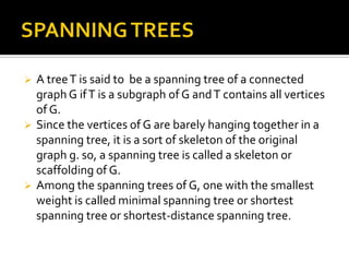
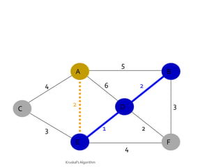
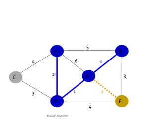
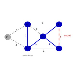
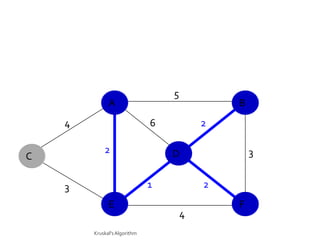
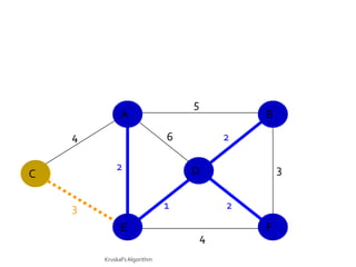
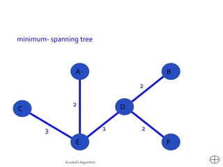
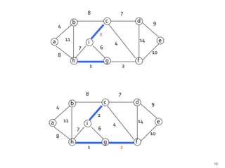
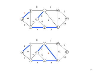
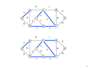
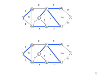
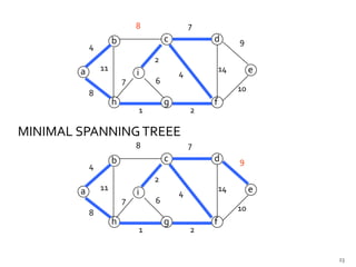
APPLICATION OF GREEDY METHOD

KRUSKAL’S ALGORITHM TO FIND
MINIMUM
        COST SPANNING TREES
   An algorithm is a mathematical procedure often used to
    solve optimization problems in a finite number of steps.

   Most solution algorithms make choices based on a
    global overview of all current and future possibilities
    aiming at reaching the single global optimum solution.

   Greedy algorithms make choices that look best at that
    every moment.
   When compared to algorithms that guarantee to yield a
    global optimum solution, greedy algorithms have
    several advantages:

   They are easier to implement, they require much less
    computing resources, they are much faster to execute.

   Their only disadvantage being that they do not always
    reach the global optimum solution
    when the global optimum solution is not
    reached, most of the times the reached sub- optimal
    solution is a very good solution.

   Several classical optimization problems like minimum
    spanning tree and optimal prefix codes for data
    compression yield global optimum solutions using
    greedy algorithm.
   A tree T is said to be a spanning tree of a connected
    graph G if T is a subgraph of G and T contains all vertices
    of G.
   Since the vertices of G are barely hanging together in a
    spanning tree, it is a sort of skeleton of the original
    graph g. so, a spanning tree is called a skeleton or
    scaffolding of G.
   Among the spanning trees of G, one with the smallest
    weight is called minimal spanning tree or shortest
    spanning tree or shortest-distance spanning tree.
A second greedy algorithm was developed by Joseph Kruskal.

Steps in Kruskal’s algorithm:
 list all edges of G in order of increasing weight.
 Select a smallest edge of G.
 For each successive step, select (from all remaining
  edges of G) another smallest edge that makes no circuit
 with the previously selected edges.
 Continue until n-1 edges have been selected.
      At each stage, the algorithm chooses an edge
     to add to its current partial solution. To do so, it needs
    to test each candidate edge (u ,v ) to
    see whether the endpoints u and v lie in different
    components; otherwise the edge produces a
    cycle.
5
              A                               B
    4                         6           2

            2                     D               3
C

    3                         1           2
              E                               F
                                      4
        Kruskal's Algorithm
enqueue edges of G in a queue in increasing order of
cost.
T=;
while(queue is not empty)
{
       dequeue an edge e;
       if(e does not create a cycle with edges in T)
       add e to T;
}
return T;
5
              A                               B
    4                         6           2

            2                     D               3
C

    3                         1           2
              E                               F
                                      4
        Kruskal's Algorithm
5
              A                               B
    4                         6           2

            2                     D               3   cycle!!
C

    3                         1           2
              E                               F
                                      4
        Kruskal's Algorithm
5
              A                               B
    4                         6           2

            2                     D               3
C

    3                         1           2
              E                               F
                                      4
        Kruskal's Algorithm
5
              A                               B
    4                         6           2

            2                     D               3
C

    3                         1           2
              E                               F
                                      4
        Kruskal's Algorithm
minimum- spanning tree


                    A                           B
                                            2

                  2                     D
C

        3                           1       2
                    E                           F

              Kruskal's Algorithm
8                   7

             b                   c           d        9
    4

                             2
        11                                       14        e
a                    i               4
                 7           6
                                                      10
    8
             h                   g           f
                         1               2
8                   7
             b                   c               d         9
    4
                             2
a       11                                           14        e
                         i           4
                 7           6
                                                          10
    8
             h                   g               f
                         1                   2


                     8                   7
             b                   c               d        9
    4
                             2
a       11                                           14        e
                     i               4
                 7           6
                                                          10
    8
             h                   g               f
                     1                   2

                                                                   19
8               7
             b               c           d        9
    4
                         2
a       11                                   14        e
                     i           4
                 7       6
                                                  10
    8
             h               g           f
                     1               2


                     8               7
             b               c           d        9
    4
                         2
a       11                                   14        e
                     i           4
                 7       6
                                                  10
    8
             h               g           f
                     1               2

                                                           20
8               7
             b               c           d        9
    4
                         2
a       11                                   14        e
                     i           4
                 7       6
                                                  10
    8
             h               g           f
                     1               2


                     8               7
             b               c           d        9
    4
                         2
a       11                                   14        e
                     i           4
                 7       6
                                                  10
    8
             h               g           f
                     1               2


                                                           21
8               7
             b               c           d        9
    4
                         2
a       11                                   14        e
                     i           4
                 7       6
                                                  10
    8
             h               g           f
                     1               2


                     8               7
             b               c           d        9
    4
                         2
a       11                                   14        e
                     i           4
                 7       6
                                                  10
    8
             h               g           f
                     1               2


                                                           22
8               7
                     b               c           d        9
            4
                                 2
        a       11                                   14        e
                             i           4
                         7       6
                                                          10
            8
                     h               g           f
                             1               2

MINIMAL SPANNING TREEE
                             8               7
                     b               c           d        9
            4
                                 2
        a       11                                   14        e
                             i           4
                         7       6
                                                          10
            8
                     h               g           f
                             1               2


                                                                   23
   Initialization O(V) time
   Sorting the edges Q(E lg E) = Q(E lg V) (why?)
   O(E) calls to FindSet
   Union costs
     Let t(v) – the number of times v is moved to a new
      cluster
     Each time a vertex is moved to a new cluster the size
      of the cluster containing the vertex at least doubles:
      t(v) log V
     Total time spent doing Union vV
                                       t (v)  V log V
   Total time: O(E lg V)
                                                               24
   Where ever the minimum distance is needed to achieve
    there this algorithm gets place.
   For example.
     In telephone lining under the ground, they have to connect all
      the cities with the minimum amount of wire.
     If the new connection is in position to add between cities, there
      we have to consider the minimum cost distance.
     Assume, if the minimum distance is not calculated, the wastage
      of wires will be in peak.
   Railways track construction.
   National highway construction.
   Flyover bridge construction.
   Network between two intranets.
   The another non-technical example will be as,
     The by-pass rider or point to point buses will move on with the
      minimum distance path to reach the destination much faster.
      They will never circulate their bus through unwanted towns and
      villages.

Application of greedy method

  • 1.
    APPLICATION OF GREEDYMETHOD KRUSKAL’S ALGORITHM TO FIND MINIMUM COST SPANNING TREES
  • 2.
    An algorithm is a mathematical procedure often used to solve optimization problems in a finite number of steps.  Most solution algorithms make choices based on a global overview of all current and future possibilities aiming at reaching the single global optimum solution.  Greedy algorithms make choices that look best at that every moment.
  • 3.
    When compared to algorithms that guarantee to yield a global optimum solution, greedy algorithms have several advantages:  They are easier to implement, they require much less computing resources, they are much faster to execute.  Their only disadvantage being that they do not always reach the global optimum solution
  • 4.
    when the global optimum solution is not reached, most of the times the reached sub- optimal solution is a very good solution.  Several classical optimization problems like minimum spanning tree and optimal prefix codes for data compression yield global optimum solutions using greedy algorithm.
  • 5.
    A tree T is said to be a spanning tree of a connected graph G if T is a subgraph of G and T contains all vertices of G.  Since the vertices of G are barely hanging together in a spanning tree, it is a sort of skeleton of the original graph g. so, a spanning tree is called a skeleton or scaffolding of G.  Among the spanning trees of G, one with the smallest weight is called minimal spanning tree or shortest spanning tree or shortest-distance spanning tree.
  • 6.
    A second greedyalgorithm was developed by Joseph Kruskal. Steps in Kruskal’s algorithm:  list all edges of G in order of increasing weight.  Select a smallest edge of G.  For each successive step, select (from all remaining edges of G) another smallest edge that makes no circuit  with the previously selected edges.  Continue until n-1 edges have been selected.
  • 7.
    At each stage, the algorithm chooses an edge to add to its current partial solution. To do so, it needs to test each candidate edge (u ,v ) to see whether the endpoints u and v lie in different components; otherwise the edge produces a cycle.
  • 8.
    5 A B 4 6 2 2 D 3 C 3 1 2 E F 4 Kruskal's Algorithm
  • 9.
    enqueue edges ofG in a queue in increasing order of cost. T=; while(queue is not empty) { dequeue an edge e; if(e does not create a cycle with edges in T) add e to T; } return T;
  • 10.
    5 A B 4 6 2 2 D 3 C 3 1 2 E F 4 Kruskal's Algorithm
  • 11.
    5 A B 4 6 2 2 D 3 C 3 1 2 E F 4 Kruskal's Algorithm
  • 12.
    5 A B 4 6 2 2 D 3 C 3 1 2 E F 4 Kruskal's Algorithm
  • 13.
    5 A B 4 6 2 2 D 3 C 3 1 2 E F 4 Kruskal's Algorithm
  • 14.
    5 A B 4 6 2 2 D 3 cycle!! C 3 1 2 E F 4 Kruskal's Algorithm
  • 15.
    5 A B 4 6 2 2 D 3 C 3 1 2 E F 4 Kruskal's Algorithm
  • 16.
    5 A B 4 6 2 2 D 3 C 3 1 2 E F 4 Kruskal's Algorithm
  • 17.
    minimum- spanning tree A B 2 2 D C 3 1 2 E F Kruskal's Algorithm
  • 18.
    8 7 b c d 9 4 2 11 14 e a i 4 7 6 10 8 h g f 1 2
  • 19.
    8 7 b c d 9 4 2 a 11 14 e i 4 7 6 10 8 h g f 1 2 8 7 b c d 9 4 2 a 11 14 e i 4 7 6 10 8 h g f 1 2 19
  • 20.
    8 7 b c d 9 4 2 a 11 14 e i 4 7 6 10 8 h g f 1 2 8 7 b c d 9 4 2 a 11 14 e i 4 7 6 10 8 h g f 1 2 20
  • 21.
    8 7 b c d 9 4 2 a 11 14 e i 4 7 6 10 8 h g f 1 2 8 7 b c d 9 4 2 a 11 14 e i 4 7 6 10 8 h g f 1 2 21
  • 22.
    8 7 b c d 9 4 2 a 11 14 e i 4 7 6 10 8 h g f 1 2 8 7 b c d 9 4 2 a 11 14 e i 4 7 6 10 8 h g f 1 2 22
  • 23.
    8 7 b c d 9 4 2 a 11 14 e i 4 7 6 10 8 h g f 1 2 MINIMAL SPANNING TREEE 8 7 b c d 9 4 2 a 11 14 e i 4 7 6 10 8 h g f 1 2 23
  • 24.
    Initialization O(V) time  Sorting the edges Q(E lg E) = Q(E lg V) (why?)  O(E) calls to FindSet  Union costs  Let t(v) – the number of times v is moved to a new cluster  Each time a vertex is moved to a new cluster the size of the cluster containing the vertex at least doubles: t(v) log V  Total time spent doing Union vV  t (v)  V log V  Total time: O(E lg V) 24
  • 25.
    Where ever the minimum distance is needed to achieve there this algorithm gets place.  For example.  In telephone lining under the ground, they have to connect all the cities with the minimum amount of wire.  If the new connection is in position to add between cities, there we have to consider the minimum cost distance.  Assume, if the minimum distance is not calculated, the wastage of wires will be in peak.
  • 26.
    Railways track construction.  National highway construction.  Flyover bridge construction.  Network between two intranets.  The another non-technical example will be as,  The by-pass rider or point to point buses will move on with the minimum distance path to reach the destination much faster. They will never circulate their bus through unwanted towns and villages.