Download to read offline
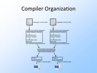
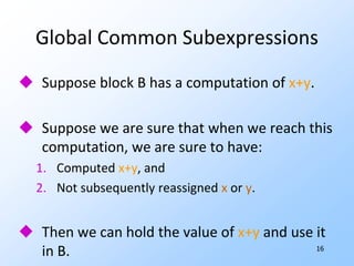
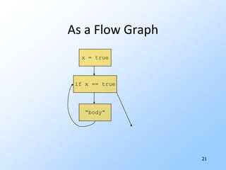
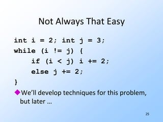
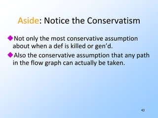
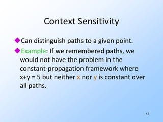
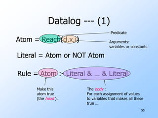
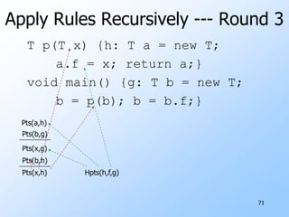
![8Intermediate Codefor (i=0; i<n; i++) A[i] = 1;Intermediate code exposes optimizable constructs we cannot see at source-code level.Make flow explicit by breaking into basic blocks = sequences of steps with entry at beginning, exit at end.](https://image.slidesharecdn.com/20101017programanalysisforsecuritylivshitslecture02compilers-101018033718-phpapp02/85/20101017-program-analysis_for_security_livshits_lecture02_compilers-10-320.jpg)
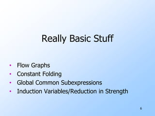
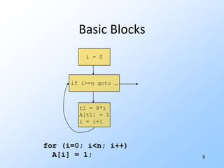
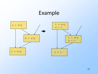
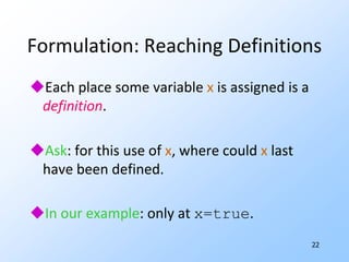
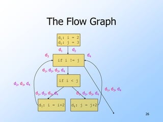
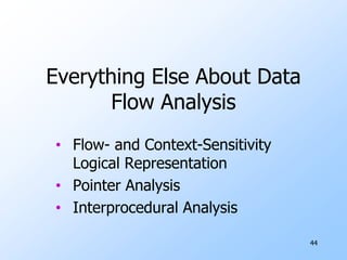
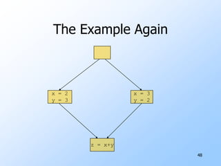
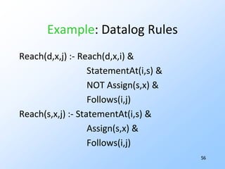
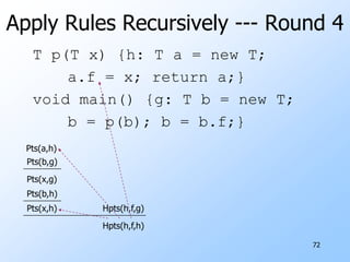
![9i = 0if i>=n goto …t1 = 8*i A[t1] = 1i = i+1 Basic Blocks for (i=0; i<n; i++) A[i] = 1;](https://image.slidesharecdn.com/20101017programanalysisforsecuritylivshitslecture02compilers-101018033718-phpapp02/85/20101017-program-analysis_for_security_livshits_lecture02_compilers-11-320.jpg)
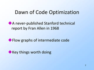
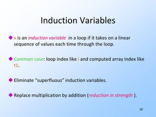
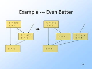
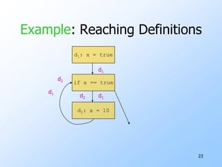
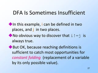
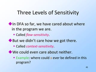
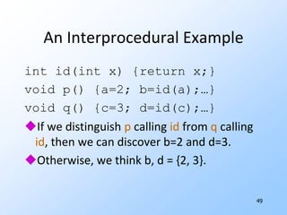
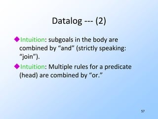
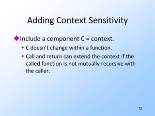
![11Examplei = 0if i>=n goto …t1 = 8*i A[t1] = 1i = i+1 t1 = 0 n1 = 8*nif t1>=n1 goto …A[t1] = 1 t1 = t1+8](https://image.slidesharecdn.com/20101017programanalysisforsecuritylivshitslecture02compilers-101018033718-phpapp02/85/20101017-program-analysis_for_security_livshits_lecture02_compilers-13-320.jpg)
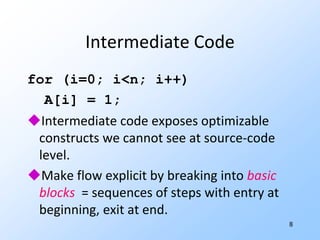
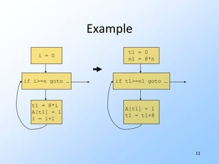
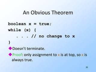
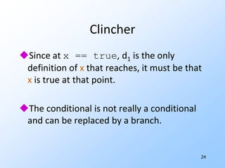
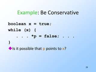
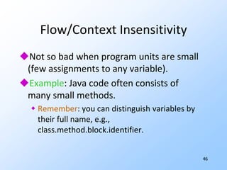
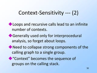
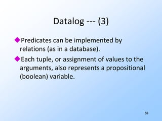
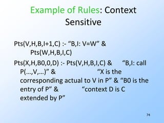
![15Examplei = 0 n = 100if i>=n goto …t1 = 8*i A[t1] = 1i = i+1 t1 = 0 if t1>=800 goto …A[t1] = 1 t1 = t1+8](https://image.slidesharecdn.com/20101017programanalysisforsecuritylivshitslecture02compilers-101018033718-phpapp02/85/20101017-program-analysis_for_security_livshits_lecture02_compilers-17-320.jpg)


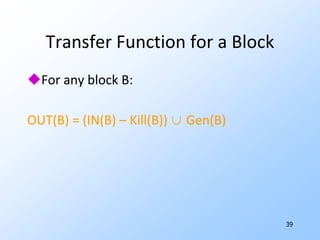
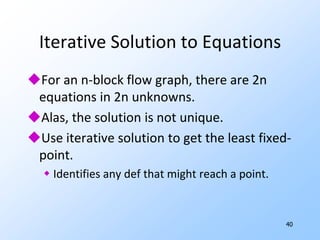
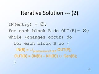
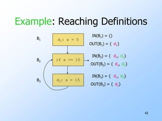
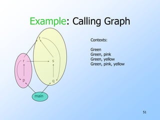
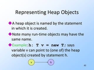
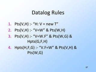

This document provides an introduction and overview of compiler optimization techniques, including: 1) Flow graphs, constant folding, global common subexpressions, induction variables, and reduction in strength. 2) Data-flow analysis basics like reaching definitions, gen/kill frameworks, and solving data-flow equations iteratively. 3) Pointer analysis using Andersen's formulation to model references between local variables and heap objects. Rules are provided to represent points-to relationships.