05 dataflow

Lecture Notes on
Dataflow Analysis
15-411: Compiler Design
Frank Pfenning
Lecture 5
September 9, 2008
1 Introduction
In this lecture we first extend liveness analysis to handle memory refer-ences
and then consider neededness analysis which is similar to liveness
and used to discover dead code. Both liveness and neededness are back-wards
dataflow analyses. We then describe reaching definitions, a forwards
dataflow analysis which is an important component of optimizations such
as constant propagation or copy propagation.
2 Memory References
Recall the rules specifying liveness analysis from the previous lecture.
use(l, x)
live(l, x)
K1
live(l0, u)
succ(l, l0)
¬def(l, u)
live(l, u)
K2
We do not repeat the rules for extracting def, use, and succ from the pro-gram.
They represent the following:
• use(l, x): the instruction at l uses variable x.
• def(l, x): the instruction at l defines (that is, writes to) variable x.
• succ(l, l0): the instruction executed after l may be l0.
LECTURE NOTES SEPTEMBER 9, 2008

L5.2 Dataflow Analysis
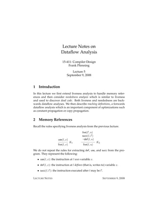
In order to model the store in our abstract assembly language, we add
two new forms of instructions
• Load: y M[x].
• Store: M[x] y.
All that is needed to extend the liveness analysis is to specify the def, use,
and succ properties of these two instructions.
l : x M[y]
def(l, x)
use(l, y)
succ(l, l0)
J6
l : M[y] x
use(l, x)
use(l, y)
succ(l, l0)
J7
The rule J7 for storing a register contents to memory does not define any
value, because liveness analysis does not track memory, only variables
which then turn into registers. Tracking memory is indeed a difficult task
and subject of a number of analyses of which alias analysis is the most
prominent. We will consider this in a later language.
The two rules for liveness itself do not need to change! This is an indi-cation
that we refactored the original specification in a good way.
3 Dead Code Elimination
An important optimization in a compiler is dead code elimination which re-moves
unneeded instructions from the program. Even if the original source
code does not contain unnecessary code, after translation to a low-level lan-guage
dead code often arises either just as an artefact of the translation itself
or as the result of optimizations. We will see an example of these phenom-ena
in Section 5; here we just use a small example.
In this code, we compute the factorial of x. The variable x is live at the
first line. This would typically be the case of an input variable to a program.
Instructions Live variables
1 : p 1 x
2 : p p x p, x
3 : z p + 1 p, x
4 : x x − 1 p, x
5 : if (x 0) goto 2 p, x
6 : return p p

Dataflow Analysis L5.3
The only unusual part of the loop is the unnecessary computation of p + 1.
We may suspect that line 3 is dead code, and we should be able to elim-inate
it, say, by replacing it with some nop instruction which has no effect,
or perhaps eliminate it entirely when we finally emit the code. The reason
to suspect this is that z is not live at the point where we define it. While
this may be sufficient reason to eliminate the assignment here, this is not
true in general. For example, we may have an assignment such as z p/x
which is required to raise an exception if x = 0, or if the result is too large
to fit into the allotted bits on the target architecture. Another example is a
memory reference such as z M[x] which is required to raise an excep-tion
if the address x has actually not been allocated or is not readable by
the executing process. We will come back to these exception in the next
section. First, we discuss another phenomenon exhibited in the following
small modification of the program above.
Instructions Live variables
1 : p 1 x, z
2 : p p x p, x, z
3 : z z + 1 p, x, z
4 : x x − 1 p, x, z
5 : if (x 0) goto 2 p, x, z
6 : return p p
Here we see that z is live in the loop (and before it) even though the value of
z does not influence the final value returned. To see this yourself, note that
in the first backwards pass we find z to be used at line 3. After computing
p, x, and z to be live at line 2, we have reconsider line 5, since 2 is one of its
successors, and add z as live to lines 5, 4, and 3.
This example shows that liveness is not precise enough to eliminate
even simple redundant instructions such as the one in line 3 above.
4 Neededness
In order to recognize that assignments as in the previous example program
are indeed redundant, we need a different property we call neededness. We
will structure the specification in the same way as we did for liveness: we
analyze each instruction and extract the properties that are necessary for
neededness to proceed without further reference to the program instruc-tions
themselves.

The crucial first idea is that the some variables are needed because an
instruction they are involved in may have an effect. Let’s call such vari-able
necessary. Formally, we write nec(l, x) to say that x is necessary at
instruction l. We use the notation for a binary operator which may raise
an exception, such as division or the modulo operator. For our set of in-structions
considered so far, the following are places where variables are
necessary because of the possiblity of effects.
l : x y z
nec(l, y)
nec(l, z)
E1
l : if (x ? c) goto l0
nec(l, x)
E2
l : return x
nec(l, x)
E3
l : y M[x]
nec(l, x)
E4
l : M[x] y
nec(l, x)
nec(l, y)
E5
Here, x is flagged as necessary at a return statement because that is the final
value returned, and a conditional branch because it is necessary to test the
condition. The effect here is either the jump, or the lack of a jump.
A side remark: on many architectures including the x86 and x86-64,
apparently innocuous instructions such as x x+y have an effect because
they set the condition code registers. This makes optimizing unstructured
machine code quite difficult. However, in compiler design we have a secret
weapon: we only have to optimize the code that we generate! For example,
if we make sure that when we compile conditionals, the condition codes
are set immediately before the branching instruction examines them, then
the implicit effects of other instructions that are part of code generation
are benign and can be ignored. However, such “benign effects” may be
lurking in unexpected places and may perhaps not be so benign after all,
so it is important to reconsider them especially as optimizations become
more aggressive.
Now that we have extracted when variables are immediately necessary
at any given line, we have to exploit this information to compute needed-ness.
We write needed(l, x) if x is needed at l. The first rule captures the
motivation for designing the rules for necessary variables.
nec(l, x)
needed(l, x)
N1
This seeds the neededness relation and we need to consider how to prop-agate
it. Our second rule is an exact analogue of the way we propagate

liveness.
needed(l0, u)
succ(l, l0)
¬def(l, u)
needed(l, u)
N2
The crucial rule is the last one. In an assignment x y z the variables y
and z are needed if x is needed in the remaining computation. If x cannot
be shown to be needed, then y and z are not needed if is an effect free
operation. Abstracting away from the particular instruction, we get the
following:
use(l, y)
def(l, x)
succ(l, l0)
needed(l0, x)
needed(l, y)
N3
We see that neededness analysis is slightly more complex than liveness
analysis: it requires three rules instead of two, and we need the new con-cept
of a variable necessary for an instruction due to effects. We can restruc-ture
the program slightly and unify the formulas nec(l, x) and needed(l, x).
This is mostly a matter of taste and modularity. Personally, I prefer to sep-arate
local properties of instructions from those that are propagated during
the analysis, because local properties are more easily re-used. The speci-fication
of neededness is actually an example of that: is employs use(l, x)
in rule N3 which we first introduced for liveness analysis. If we had struc-tured
liveness analysis so that the rules for instructions generate live(l, x)
directly, it would not have worked as well here.
We can now perform neededness analysis on our example program. We
have indexed each variable with the numbers of all rules that can be used
to infer that they are needed (N1, N2, or N3).
Instructions Needed variables
1 : p 1 x2
2 : p p x p3, x2,3
3 : z z + 1 p2, x2
4 : x x − 1 p2, x3
5 : if (x 0) goto 2 p2, x1,2
6 : return p p1
At the crucial line 3, z is defined but not needed on line 4, and consequently
it is not needed at line 3 either.

Since the right-hand side of z z + 1 does not have an effect, and z
is not needed at any successor line, this statement is dead code and can be
optimized away.
5 Reaching Definitions
The natural direction for both liveness analysis and neededness analysis
is to traverse the program backwards. In this section we present another
important analysis whose natural traversal directions is forward. As moti-vating
example for this kind of analysis we use an array access with bounds
checks.
We imagine in our source language (which remains nebulous for the
time being) we have an assignment x = A[0] where A is an array. We
also assume there are (assembly language) variables n with the number of
elements in array A, s with the size of the array elements, and a with the
base address of the array. We might then translate the assignment to the
following code:
1 : i 0
2 : if (i 0) goto error
3 : if (i n) goto error
4 : t i s
5 : u a + t
6 : x M[u]
7 : return x
The last line is just to create a live variable x. We notice that line 2 is redun-dant
because the test will always be false. We do this in two steps. First we
apply constant propagation to replace (i 0) by (0 0) and then apply con-stant
folding to evaluate the comparison to 0 (representing falsehood). Line
3 is necessary unless we know that n 0. Line 4 performs a redundant
multiplication: because i is 0 we know t must also be 0. This is an example
of an arithmetic optimization similar to constant folding. And now line 5
is a redundant addition of 0 and can be turned into a move u a, again a
simplification of modular arithmetic.

At this point the program has become
1 : i 0
2 : nop
3 : if (i n) goto error
4 : t 0
5 : u a
6 : x M[u]
7 : return x
Now we notice that line 4 is dead code because t is not needed. We can also
apply copy propagation to replace M[u] by M[a], which now makes u not
needed so we can apply dead code elimination to line 4. Finally, we can again
apply constant propagation to replace the only remaining occurrence of i in
line 3 by 0 followed by dead code elimination for line 1 to obtain
1 : nop
2 : nop
3 : if (0 n) goto error
4 : nop
5 : nop
6 : x M[a]
7 : return x
which can be quite a bit more efficient than the first piece of code. Of course,
when emitting machine code we can delete the nop operations to reduce
code size.
One important lesson from this example is that many different kinds of
optimizations have to work in concert in order to produce efficient code in
the end. What we are interested in for this lecture is what properties we
need for the code to ensure that the optimization are indeed applicable.
We return to the very first optimization. We replaced the test (i 0)
with (0 0). This looks straightforward, but what happens if some other
control flow path can reach the test? For example, we can insert an incre-

ment and a conditional to call this optimization into question.
1 : i 0 1 : i 0
2 : if (i 0) goto error 2 : if (i 0) goto error
3 : if (i n) goto error 3 : if (i n) goto error
4 : t i s 4 : t i s
5 : u a + t 5 : u a + t
6 : x M[u] 6 : x M[u]
7 : return x 7 : i i + 1
8 : if (i n) goto 2
9 : return x
Even though lines 1–6 have not changed, suddenly we can no longer re-place
(i 0) with (0 0) because the second time line 2 is reached, i is
1. With arithmetic reasoning we may be able to recover the fact that line
2 is redundant, but pure constant propogation and constant folding is no
longer sufficient.
What we need to know is that the definition of i in line 1 is the only
definition of i that can reach line 2. This is true in the program on the left,
but not on the right since the definition of i at line 7 can also reach line 2 if
the condition at line 9 is true.
We say a definition l : x . . . reaches a line l0 if there is a path of control
flow from l to l0 at which x is not redefined. In logical language:
• reaches(l, x, l0) if the definition of x at l reaches l0.
We only need two inference rules to defines this analysis. The first states
that a variable definition reaches any immediate successor. The second ex-presses
that we can propagate a reaching definition of x to all successors of
a line l0 we have already reached, unless this line also defines x.
def(l, x)
succ(l, l0)
reaches(l, x, l0)
R1
reaches(l, x, l0)
succ(l0, l00)
¬def(l0, x)
reaches(l, x, l00)
R2
Analyzing the original program on the left, we see that the definition of
i at line 1 reaches lines 2–7, and this is (obviously) the only definition of i
reching lines 2 and 4. We can therefore apply the optimizations sketched
above.
In the program on the right hand side, the definition of i at line 7 also
reaches lines 2–8 so neither optimization can be applied.

Inspection of rule R2 confirms the intuition that reaching definitions are
propagated forward along the control flow edges. Consequently, a good im-plementation
strategy starts at the beginning of a program and computes
reaching definitions in the forward direction. Of course, saturation in the
presence of backward branches means that we may have to reconsider ear-lier
lines, just as in the backwards analysis.
A word on complexity: we can bound the size of the saturated database
for reaching definitions by L2, where L is the number of lines in the pro-gram.
This is because each line defines at most one variable (or, in realistic
machine code, a small constant number). Counting prefix firings (which
we have not yet discussed) does not change this estimate, and we obtain a
complexity of O(L2). This is not quite as efficient as liveness or neededness
analysis (which are O(L·V )), so we may need to be somewhat circumspect
in computing reaching definitions.
6 Summary
We have extended the ideas behind liveness analysis to neededness anal-ysis
which enables more aggressive dead code elimination. Neededness
is another example of a program analysis proceeding naturally backward
through the program, iterating through loops.
We have also seen reaching definitions, which is a forward dataflow
analysis necessary for a number of important optimizations such as con-stant
propagation or copy propagation. Reaching definitions can be spec-ified
in two rules and do not require any new primitive concepts beyond
variable definitions (def(x, l)) and the control flow graph (succ(l, l0)), both
of which we already needed for liveness analysis.
For an alternative approach to dataflow analysis via dataflow equations,
see the textbook [App98], Chapters 10.1 and 17.1–3. Notes on implementa-tion
of dataflow analyses are in Chapter 10.1–2 and 17.4. Generally speak-ing,
a simple iterative implementation with a library data structure for sets
which traverses the program in the natural direction should be efficient
enough for our purposes. We would advise against using bitvectors for
sets. Not only are the sets relatively sparse, but bitvectors are more time-consuming
to implement. An interesting alternative to iterating over the
program, maintaining sets, is to do the analysis one variable at a time (see
the remark on page 216 of the textbook). The implementation via a saturat-ing
engine for Datalog is also interesting, a bit more difficult to tie into the
infrastructure of a complete compiler. The efficiency gain noted by Whaley

et al. [WACL05] becomes only critical for interprocedural and whole pro-gram
analyses rather than for the intraprocedural analyses we have pre-sented
so far.
References
[App98] Andrew W. Appel. Modern Compiler Implementation in ML.
Cambridge University Press, Cambridge, England, 1998.
[WACL05] John Whaley, Dzintars Avots, Michael Carbin, and Monica S.
Lam. Using Datalog and binary decision diagrams for program
analysis. In K.Yi, editor, Proceedings of the 3rd Asian Symposium
on Programming Languages and Systems (APLAS’05), pages 97–
118. Springer LNCS 3780, November 2005.

05 dataflow

More Related Content

What's hot

Viewers also liked

Similar to 05 dataflow

Recently uploaded

05 dataflow