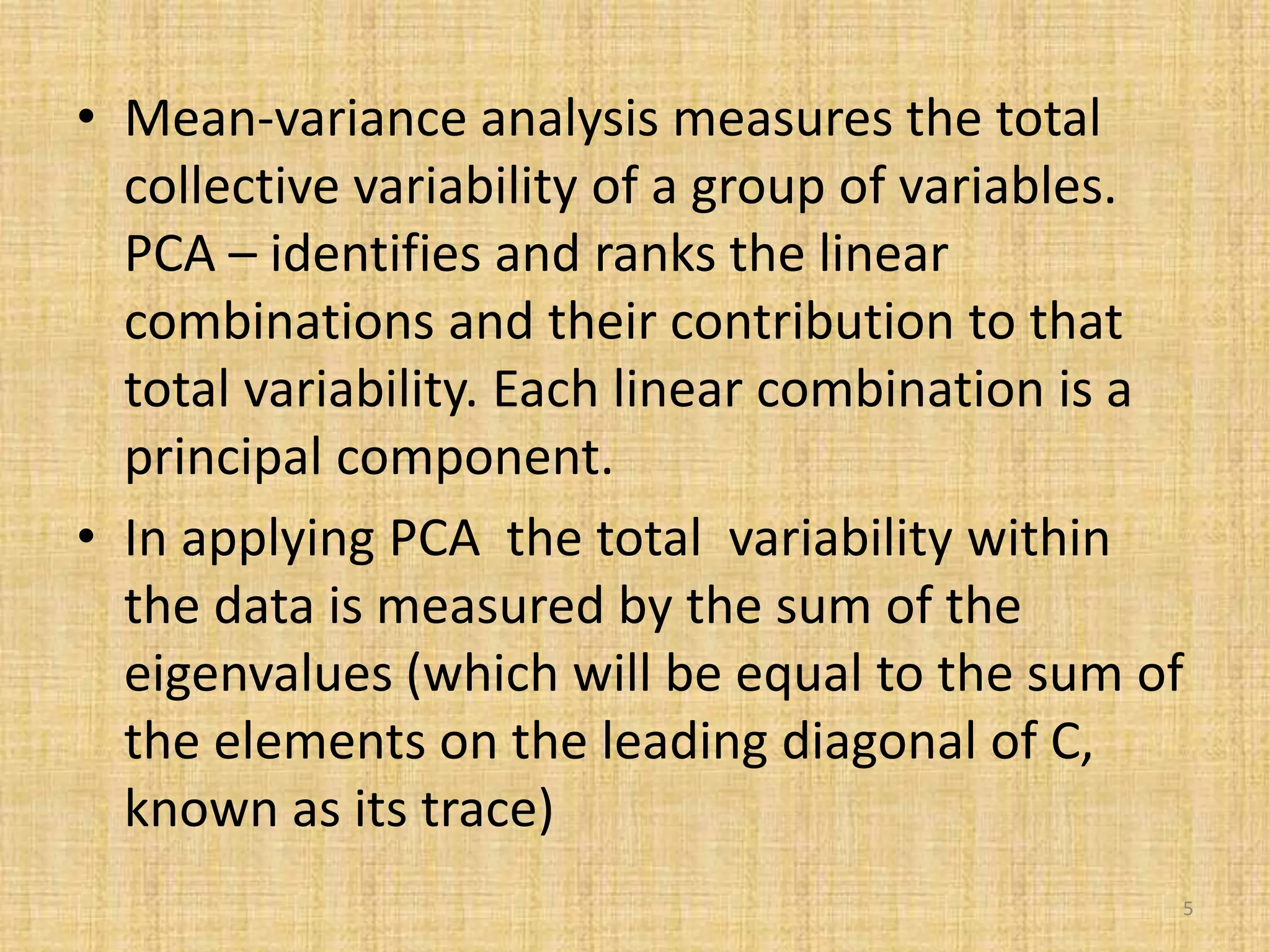
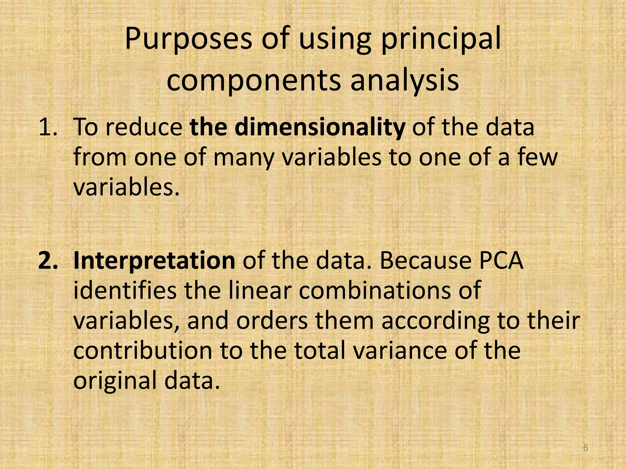
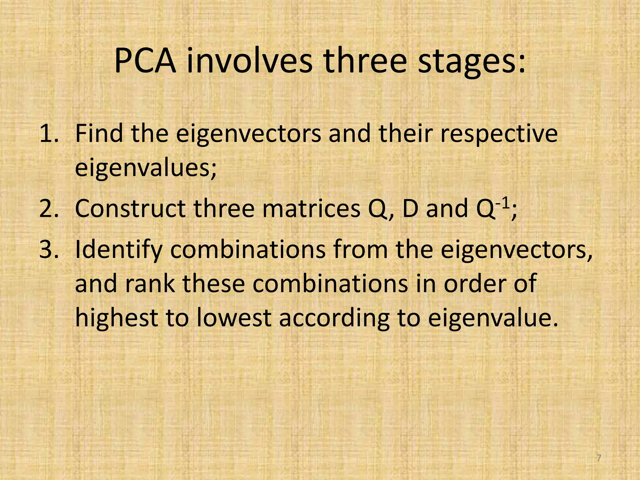
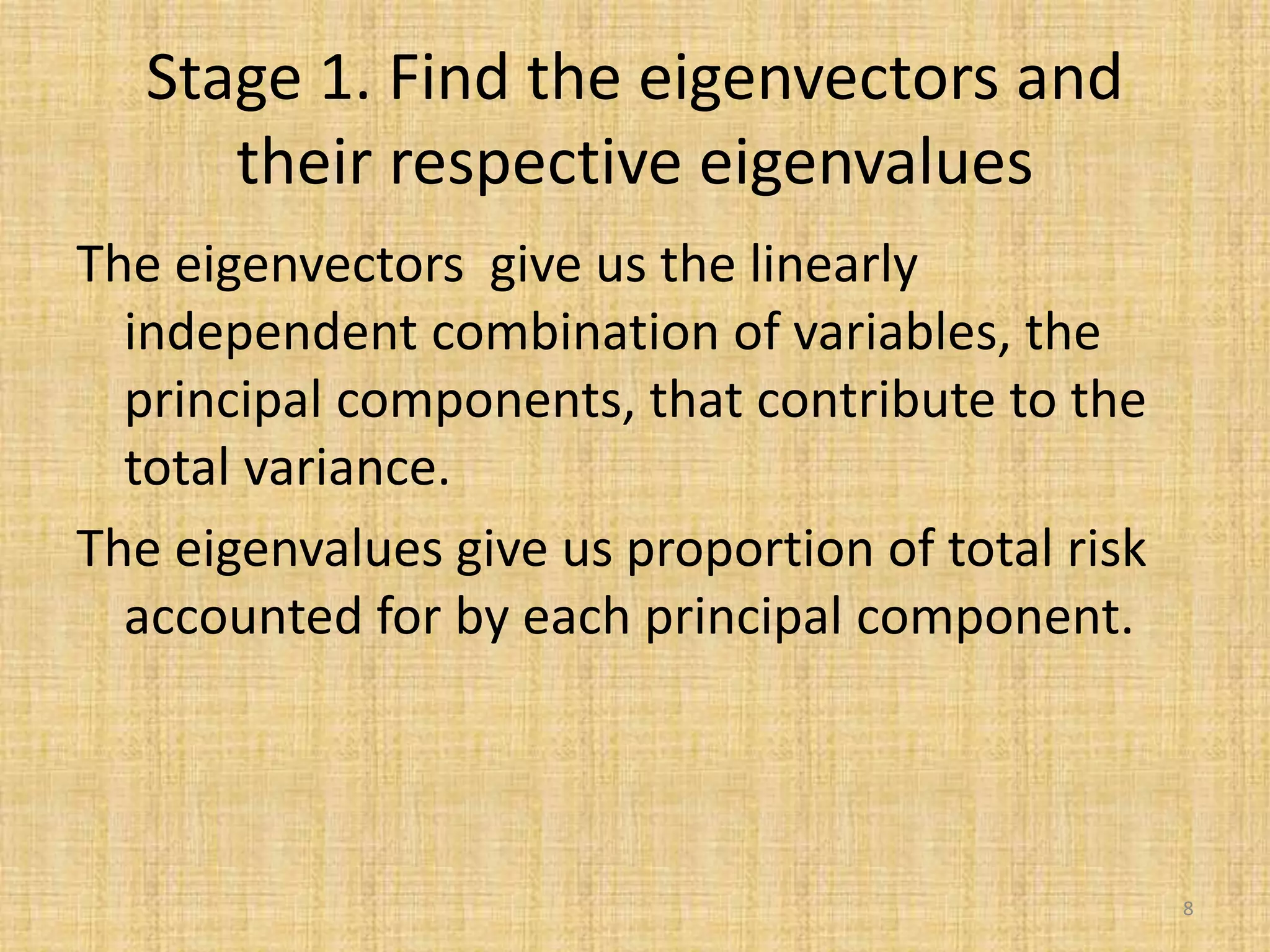
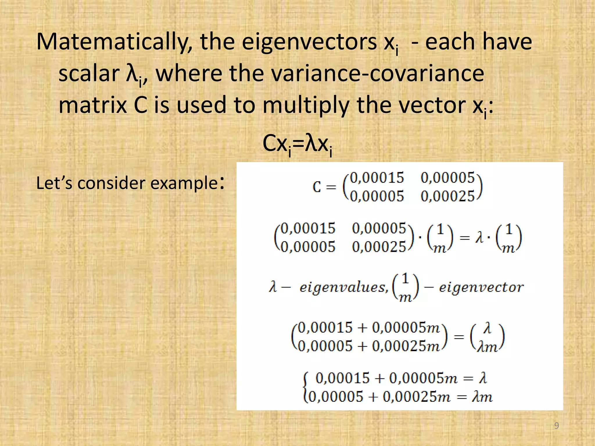
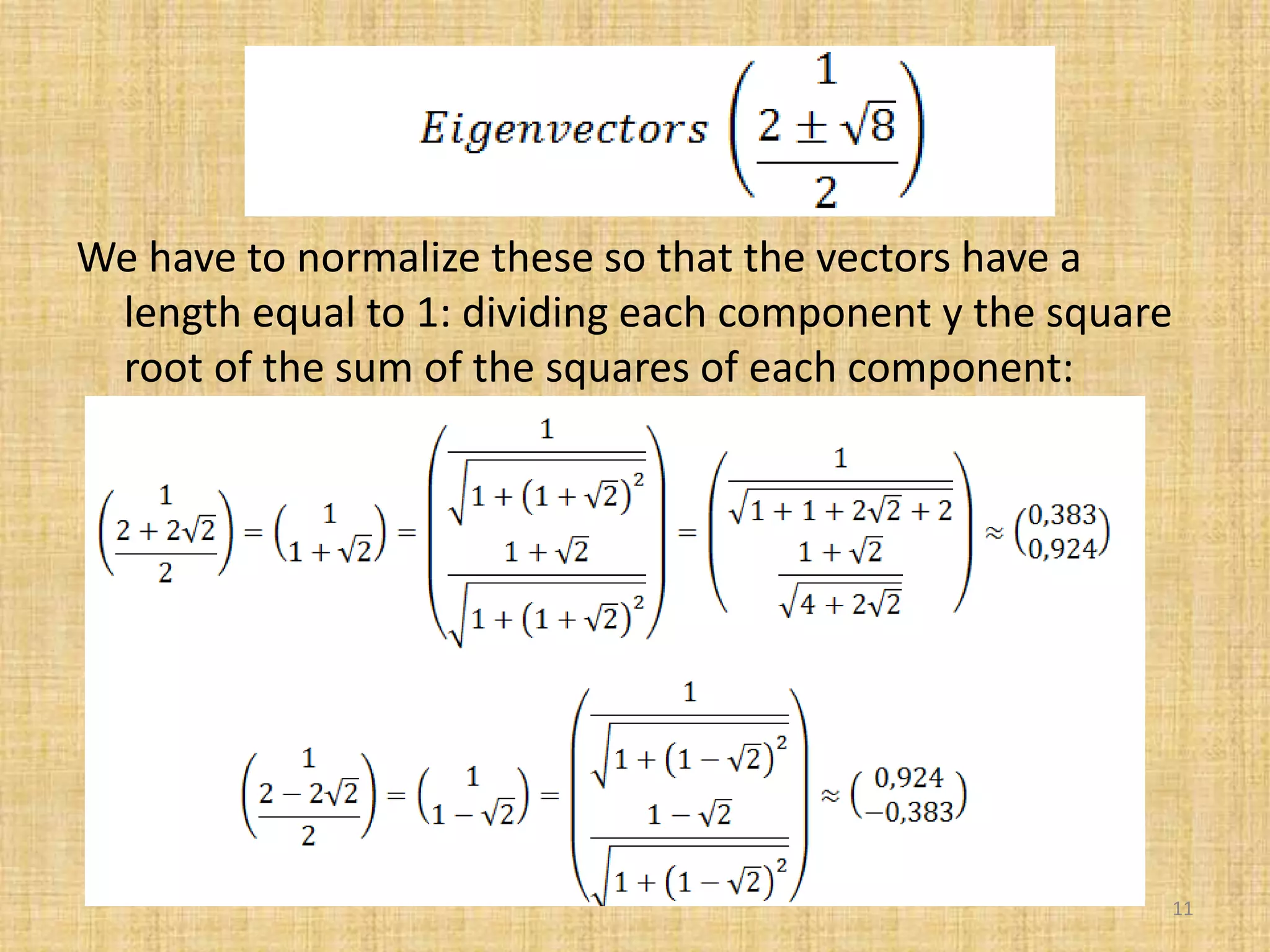
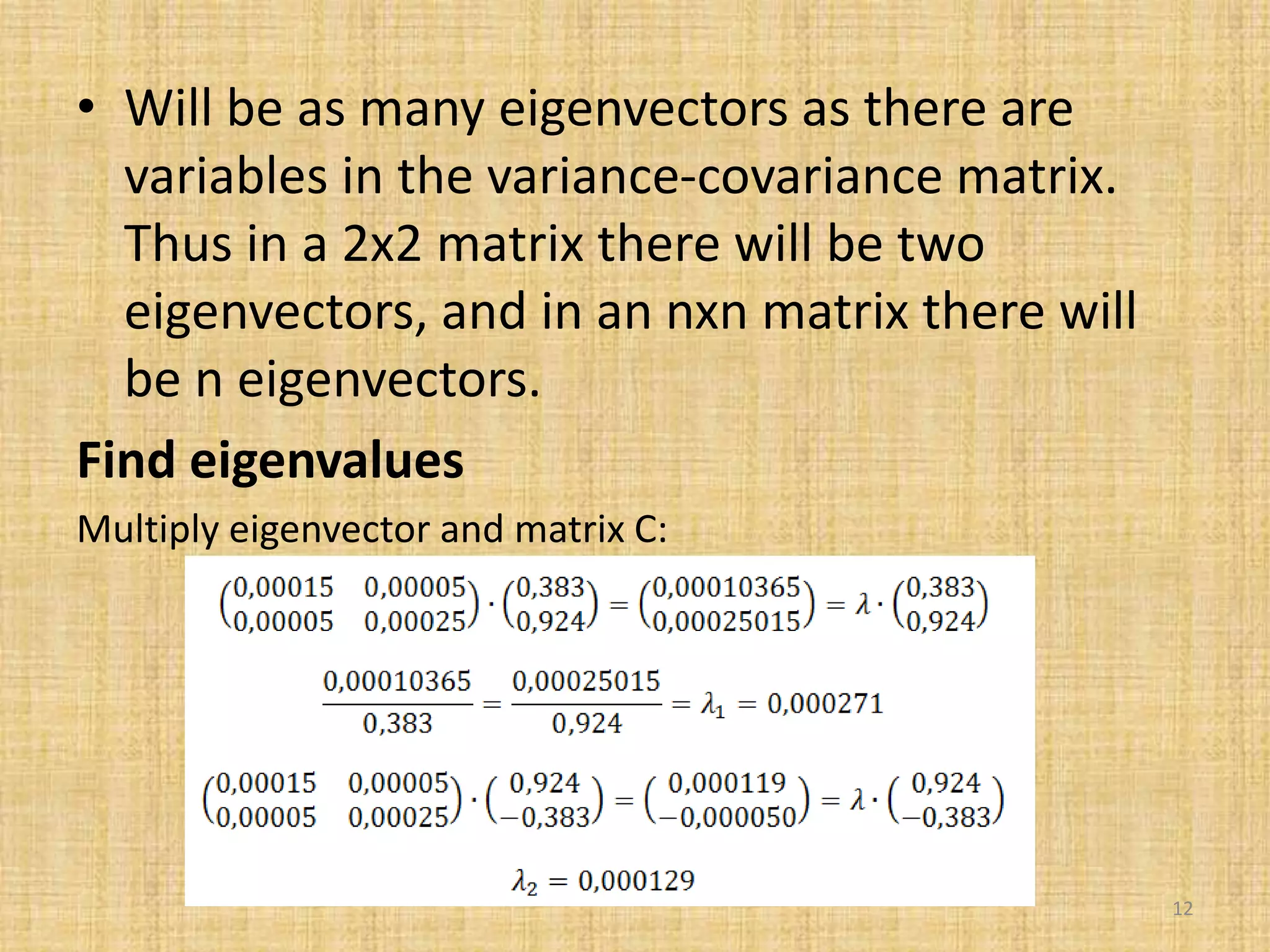
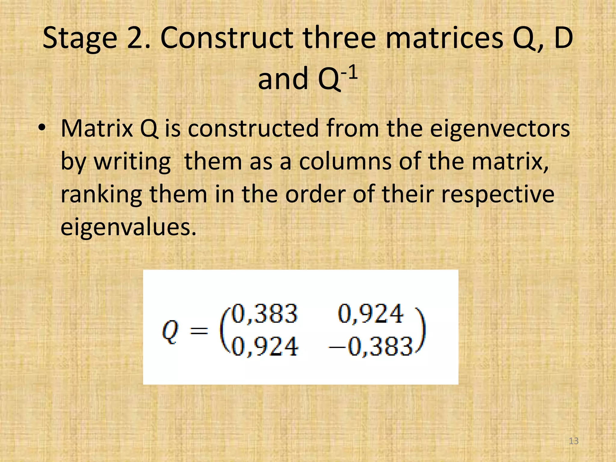
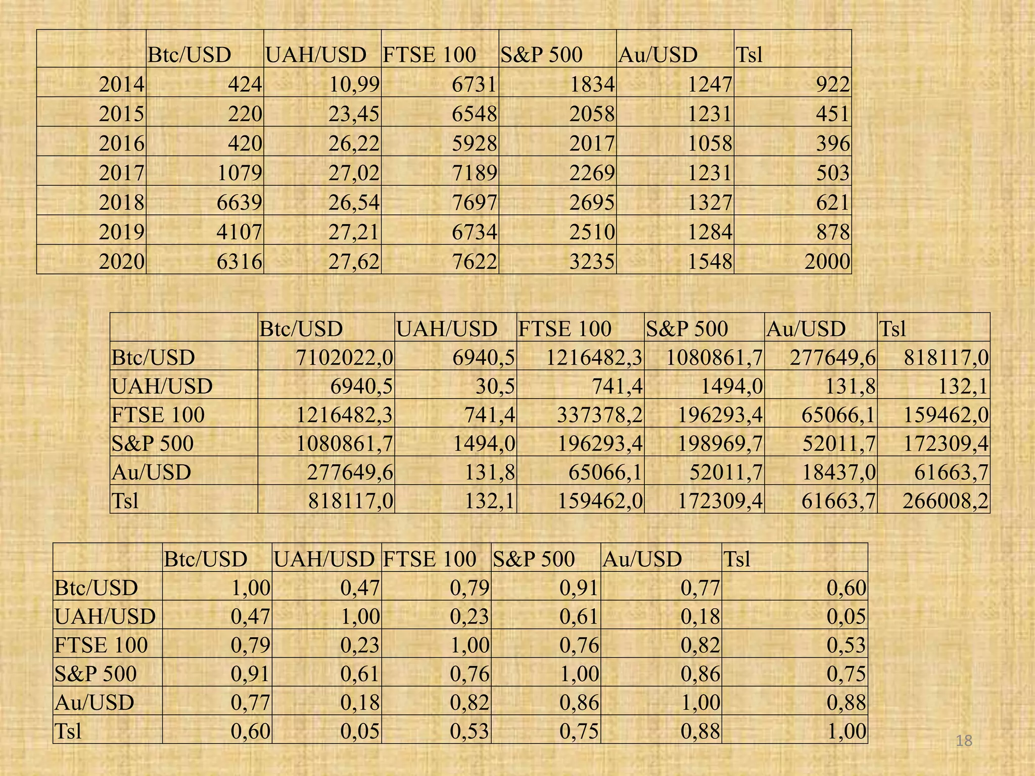
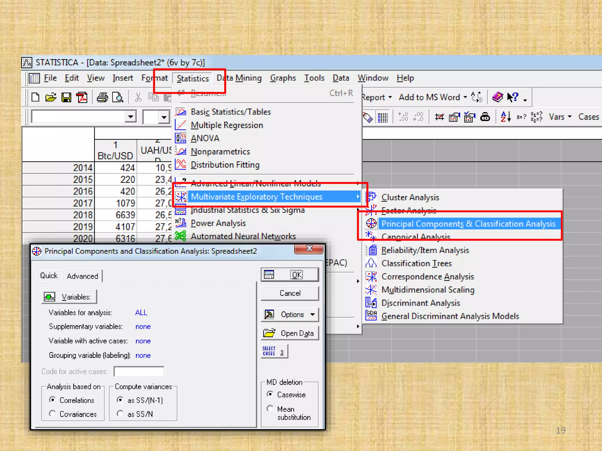
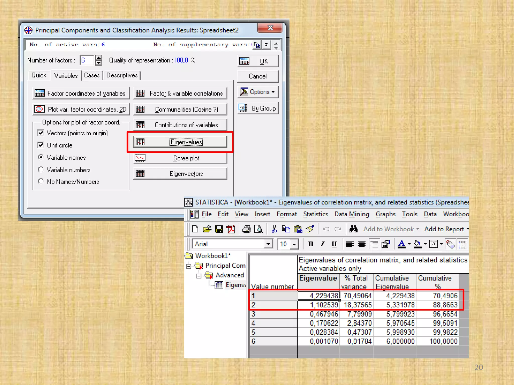
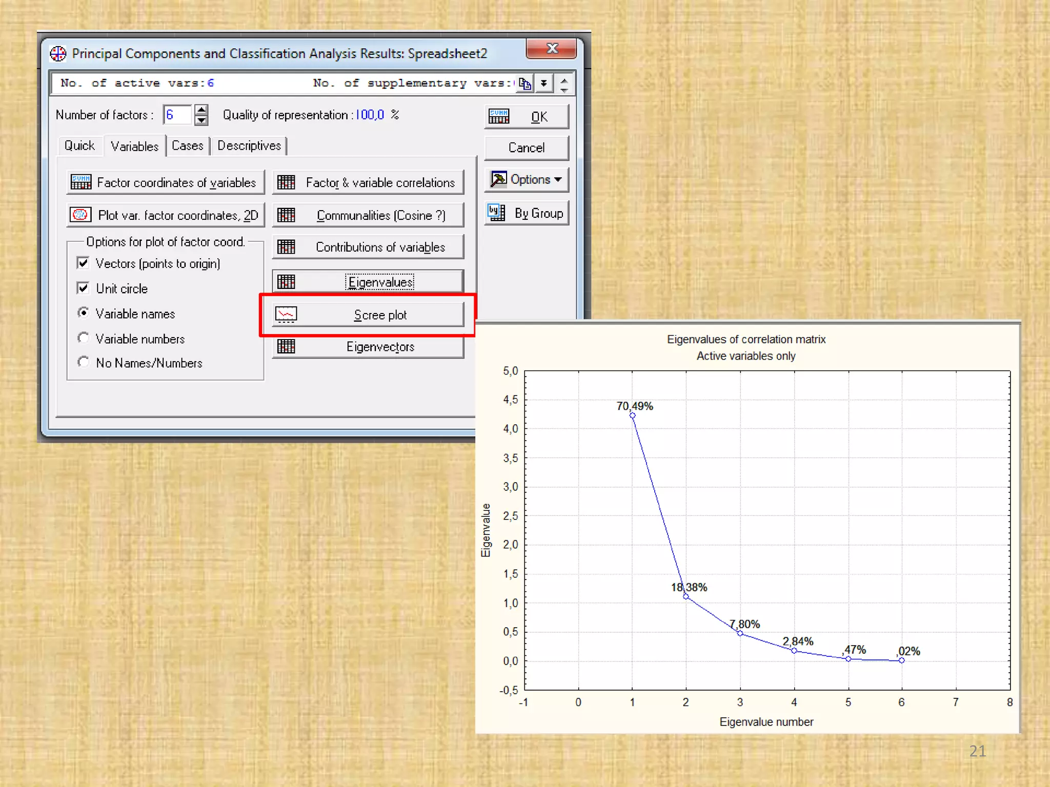
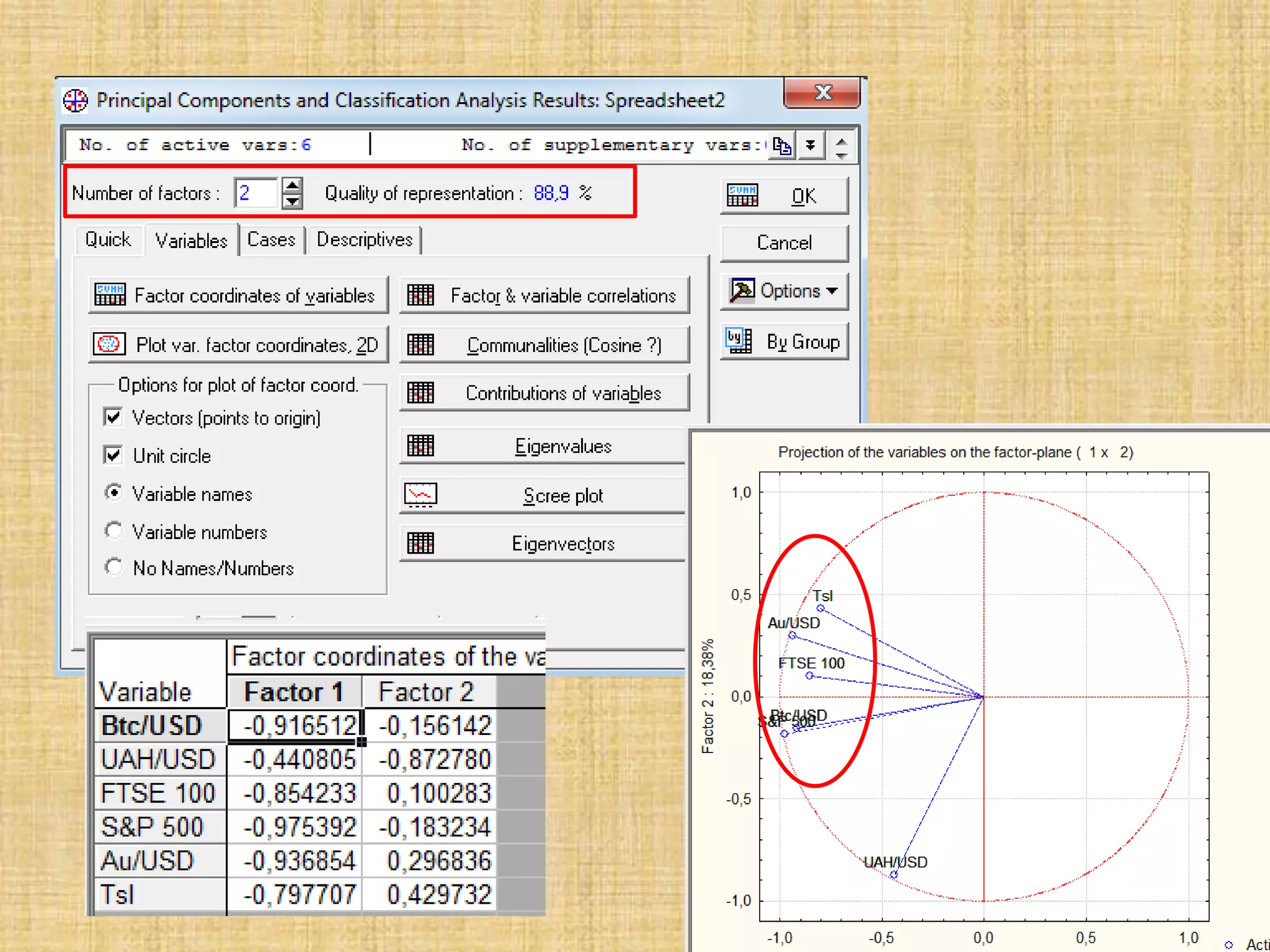
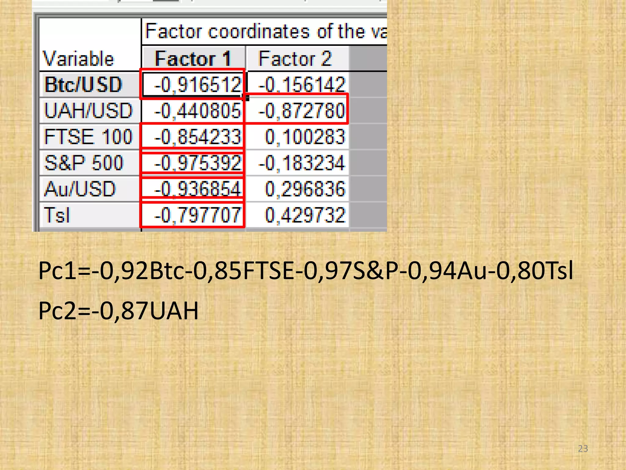
The document discusses multivariate analysis techniques, specifically principal components analysis (PCA) and factor analysis (FA), emphasizing their application in understanding data structure. It outlines the stages of PCA, including finding eigenvectors and eigenvalues, constructing matrices, and identifying ranked combinations of variables. Additionally, it highlights the purpose of PCA in reducing data dimensionality and interpreting variance in datasets.

1. Multivariate analysis: principal
components analysis and factor
analysis
Kashcha Mariya
1

2. Contents
• Introduction
• Principal components analysis
• Application of principal components analysis
2

3. Introduction
Principal components analysis and factor
analysis are techniques for analyzing the
structure of data within a multivariate
framework. In this case the structure of the
relationship between the endogenous
variables only is investigated.
One difficulty is to determine which of the
variables to include in the structure and
therefore which variables to measure.
3

4. • Principal components analysis (PCA) is used
the volatility of a multivariate structure is
being analyzed.
• Factor analysis (FA) is used when the
correlation between the variables of a
multivariate structure is being analyzed.
• Both rely on analyzing the variance/covariance
matrix(C).
4

5. • Mean-variance analysis measures the total
collective variability of a group of variables.
PCA – identifies and ranks the linear
combinations and their contribution to that
total variability. Each linear combination is a
principal component.
• In applying PCA the total variability within
the data is measured by the sum of the
eigenvalues (which will be equal to the sum of
the elements on the leading diagonal of C,
known as its trace)
5

6. Purposes of using principal
components analysis
1. To reduce the dimensionality of the data
from one of many variables to one of a few
variables.
2. Interpretation of the data. Because PCA
identifies the linear combinations of
variables, and orders them according to their
contribution to the total variance of the
original data.
6

7. PCA involves three stages:
1. Find the eigenvectors and their respective
eigenvalues;
2. Construct three matrices Q, D and Q-1;
3. Identify combinations from the eigenvectors,
and rank these combinations in order of
highest to lowest according to eigenvalue.
7

8. Stage 1. Find the eigenvectors and
their respective eigenvalues
The eigenvectors give us the linearly
independent combination of variables, the
principal components, that contribute to the
total variance.
The eigenvalues give us proportion of total risk
accounted for by each principal component.
8

9. Matematically, the eigenvectors xi - each have
scalar λi, where the variance-covariance
matrix C is used to multiply the vector xi:
Cxi=λxi
Let’s consider example:
9

10. 10

11. We have to normalize these so that the vectors have a
length equal to 1: dividing each component y the square
root of the sum of the squares of each component:
11

12. • Will be as many eigenvectors as there are
variables in the variance-covariance matrix.
Thus in a 2x2 matrix there will be two
eigenvectors, and in an nxn matrix there will
be n eigenvectors.
Find eigenvalues
Multiply eigenvector and matrix C:
12

13. Stage 2. Construct three matrices Q, D
and Q-1
• Matrix Q is constructed from the eigenvectors
by writing them as a columns of the matrix,
ranking them in the order of their respective
eigenvalues.
13

14. • Matrix D is a diagonal matrix, the diagonal
elements being the eigenvalues written in the
same order as the eigenvectors in Q:
14

15. CQ=QD / ∙ Q-1
CQ ∙ Q-1 =QDQ-1
CQ ∙ Q-1 =QDQ-1
C=QDQ-1
15

16. Stage 3. Identify combinations of
variables and rank these combinations
according to eigenvalue.
Consider the variance/covariance matrix from
two assets X and Y. The variance of this two-
asset portfolio can be written as:
16

17. 17
First principal component
Second main component
(corresponds to the smaller eigenvalue)
Total variance equal sum of eigenvalues:
D=0,000271+0,000129=0,0004
First eigenvector contributes:
0,000271/0,0004=0,6775=67,75% of the total variance

18. 18
Btc/USD UAH/USD FTSE 100 S&P 500 Au/USD Tsl
2014 424 10,99 6731 1834 1247 922
2015 220 23,45 6548 2058 1231 451
2016 420 26,22 5928 2017 1058 396
2017 1079 27,02 7189 2269 1231 503
2018 6639 26,54 7697 2695 1327 621
2019 4107 27,21 6734 2510 1284 878
2020 6316 27,62 7622 3235 1548 2000
Btc/USD UAH/USD FTSE 100 S&P 500 Au/USD Tsl
Btc/USD 1,00 0,47 0,79 0,91 0,77 0,60
UAH/USD 0,47 1,00 0,23 0,61 0,18 0,05
FTSE 100 0,79 0,23 1,00 0,76 0,82 0,53
S&P 500 0,91 0,61 0,76 1,00 0,86 0,75
Au/USD 0,77 0,18 0,82 0,86 1,00 0,88
Tsl 0,60 0,05 0,53 0,75 0,88 1,00
Btc/USD UAH/USD FTSE 100 S&P 500 Au/USD Tsl
Btc/USD 7102022,0 6940,5 1216482,3 1080861,7 277649,6 818117,0
UAH/USD 6940,5 30,5 741,4 1494,0 131,8 132,1
FTSE 100 1216482,3 741,4 337378,2 196293,4 65066,1 159462,0
S&P 500 1080861,7 1494,0 196293,4 198969,7 52011,7 172309,4
Au/USD 277649,6 131,8 65066,1 52011,7 18437,0 61663,7
Tsl 818117,0 132,1 159462,0 172309,4 61663,7 266008,2

19. 19

20. 20

21. 21

22. 22

23. Pc1=-0,92Btc-0,85FTSE-0,97S&P-0,94Au-0,80Tsl
Pc2=-0,87UAH
23

24. Laboratory work 7
• Repeat the research conducted in the lecture,
adding at your discretion one (or more)
indicators that correlate with the exchange
rate of the UAH (in relation to USD)
24

25. • StatQuest: Principal Component Analysis
(PCA), Step-by-Step
25