Downloaded 64 times

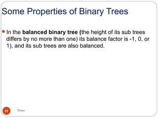
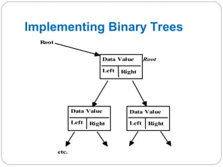
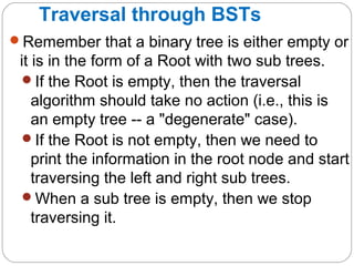
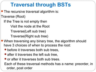
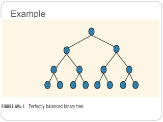
![Some Properties of Binary Trees
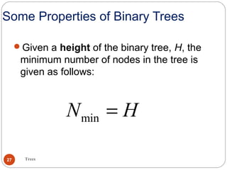
The minimum height of a binary tree is determined
as follows:
[ ]min 2log 1H N= +
Trees26
For instance, if there are three nodes to be
stored in the binary tree (N=3) then Hmin=2.](https://image.slidesharecdn.com/lecture5trees-140719095213-phpapp01/85/Lecture-5-trees-26-320.jpg)
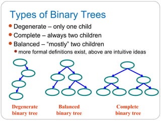

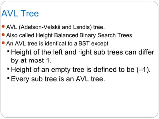
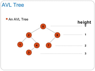
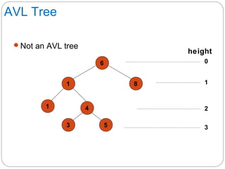

The document discusses trees as a data structure. It begins by defining basic tree concepts such as nodes, branches, degrees of nodes, roots, leaves, internal nodes, parents, children, siblings, ancestors, descendants, paths, levels, heights, and subtrees. It then discusses binary trees specifically and their properties including traversal methods. Finally, it covers balanced binary search trees and techniques for maintaining balance such as rotations during insertions and deletions.