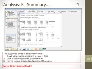
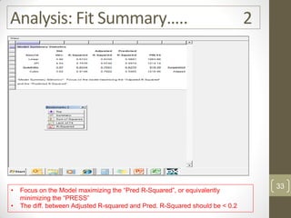
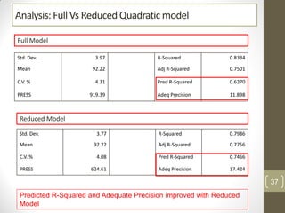
The reduced model is better than the full model based on the following criteria:
1. The reduced model has a higher R-squared and adjusted R-squared value indicating it fits the data better.
2. The predicted R-squared of the reduced model is closer to the adjusted R-squared indicating it has better predictive power.
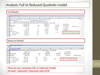
3. The PRESS value which indicates prediction accuracy is lower for the reduced model.
4. The lack of fit F-value is higher (better) for the reduced model indicating it fits the data as well as the full quadratic model without the extra terms.
Therefore, the reduced model is more statistically significant and has better predictive ability compared to the full quadratic model based on these


![谷歌留痕技术 [ 𝙩𝙤𝙥 𝟮𝟯𝟯. 𝙘 𝙤𝙢 ]](https://cdn.slidesharecdn.com/ss_thumbnails/top233-260130174328-3833018c-thumbnail.jpg?width=640&height=640&fit=bounds)


