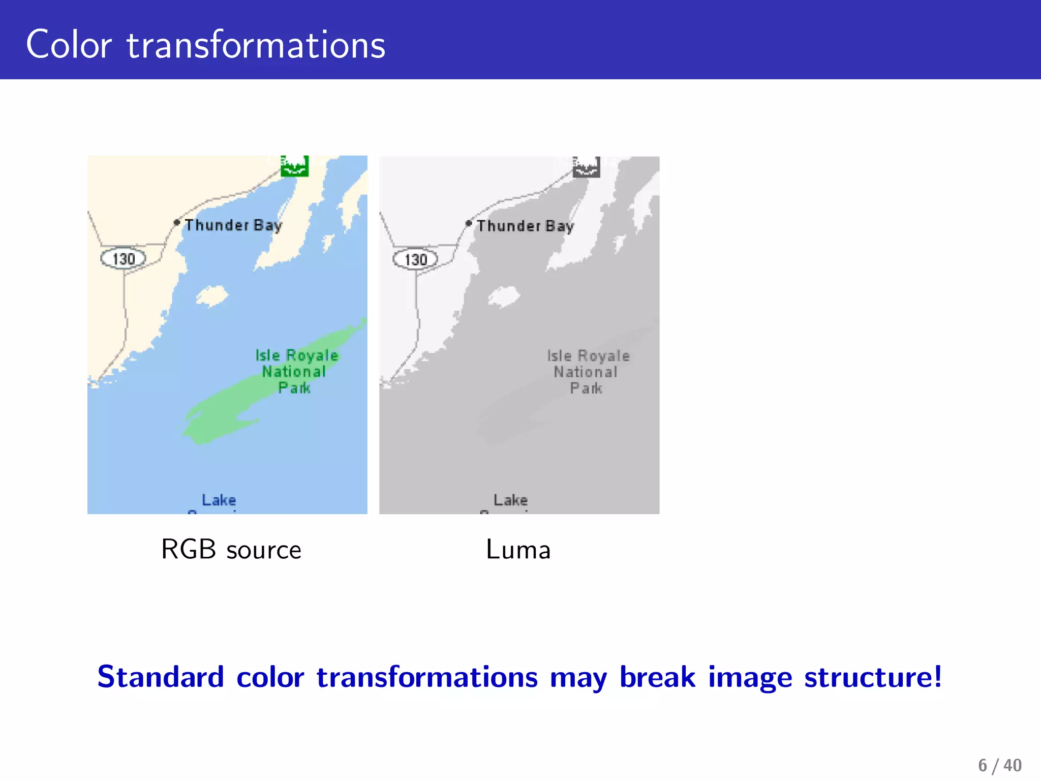
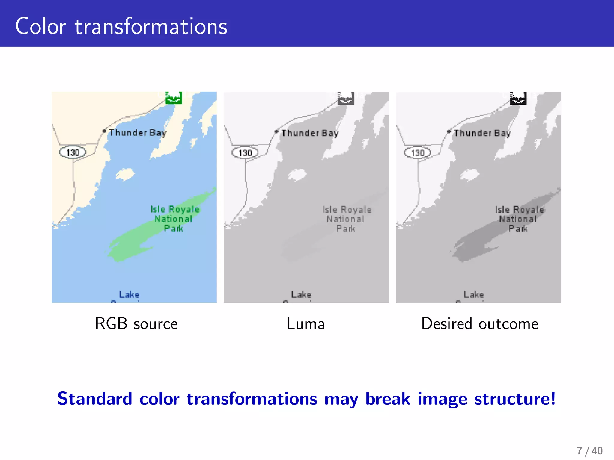
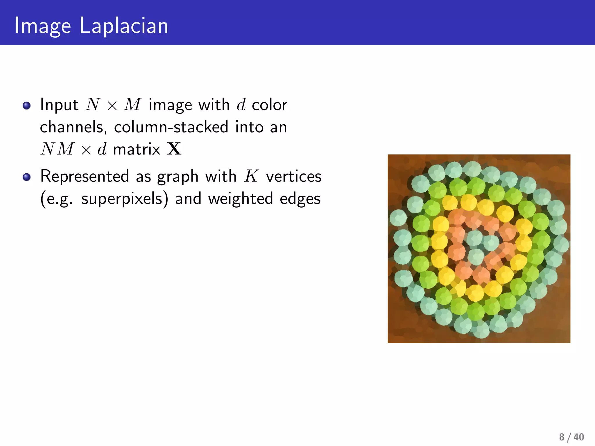
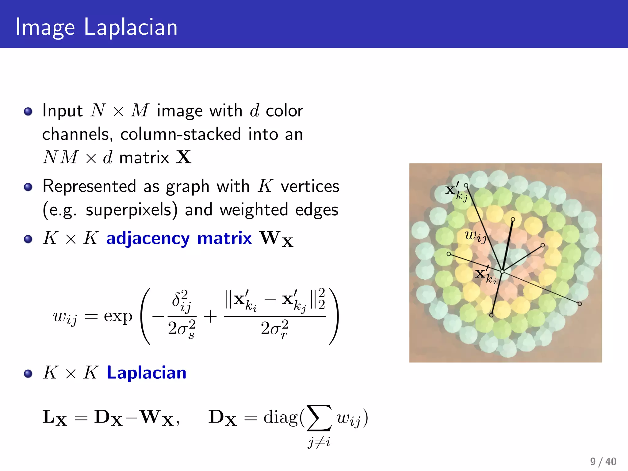
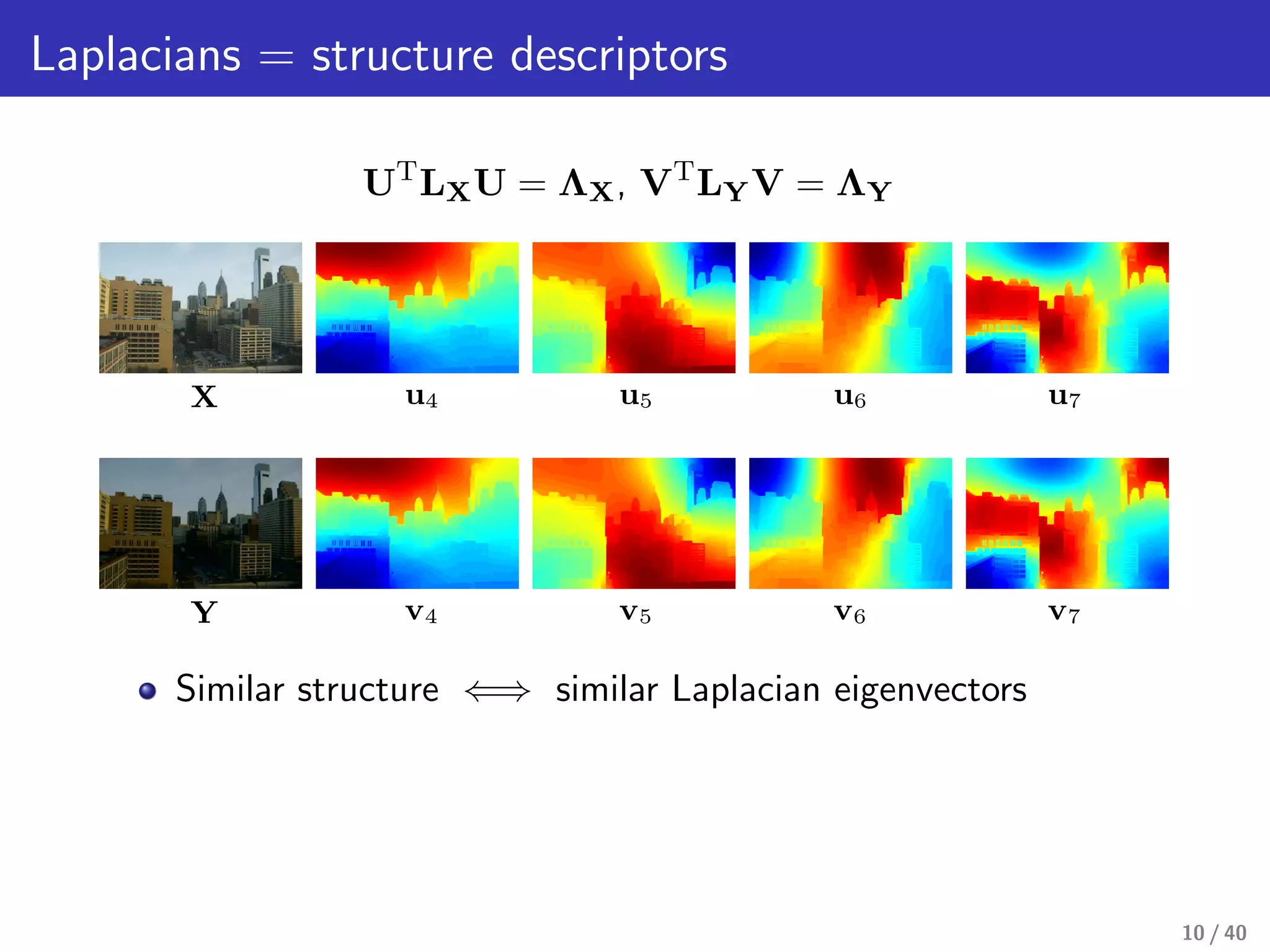
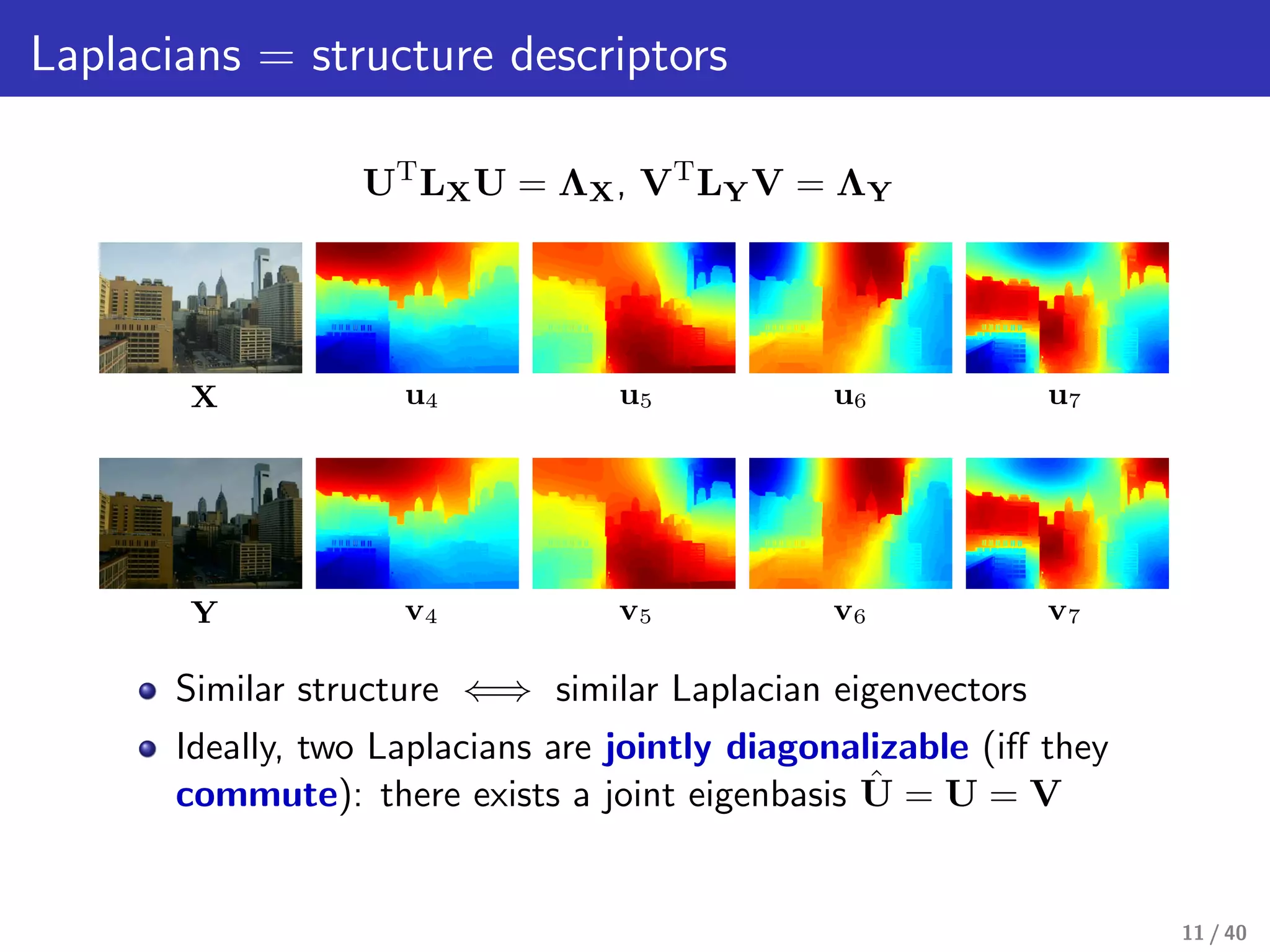
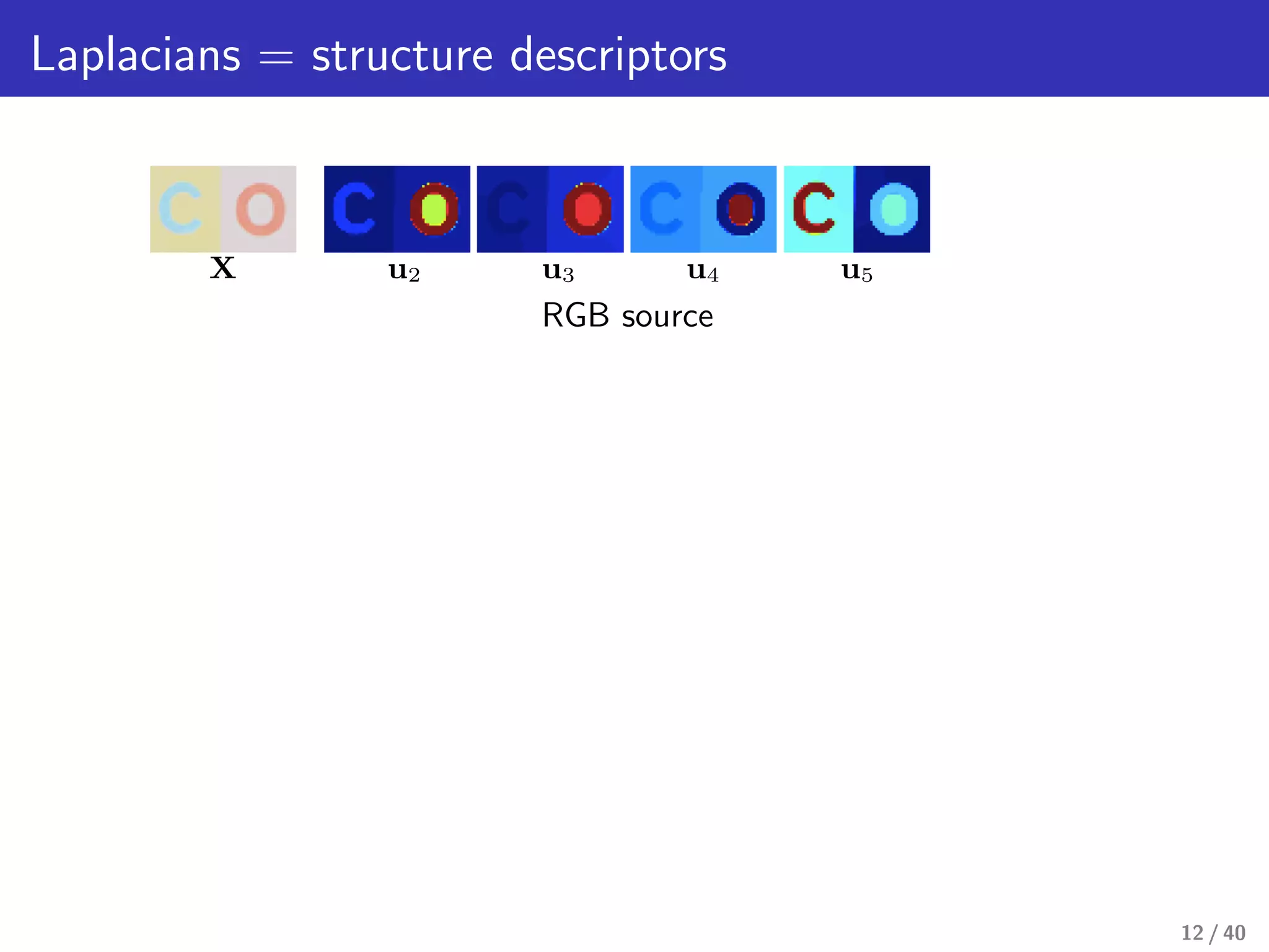
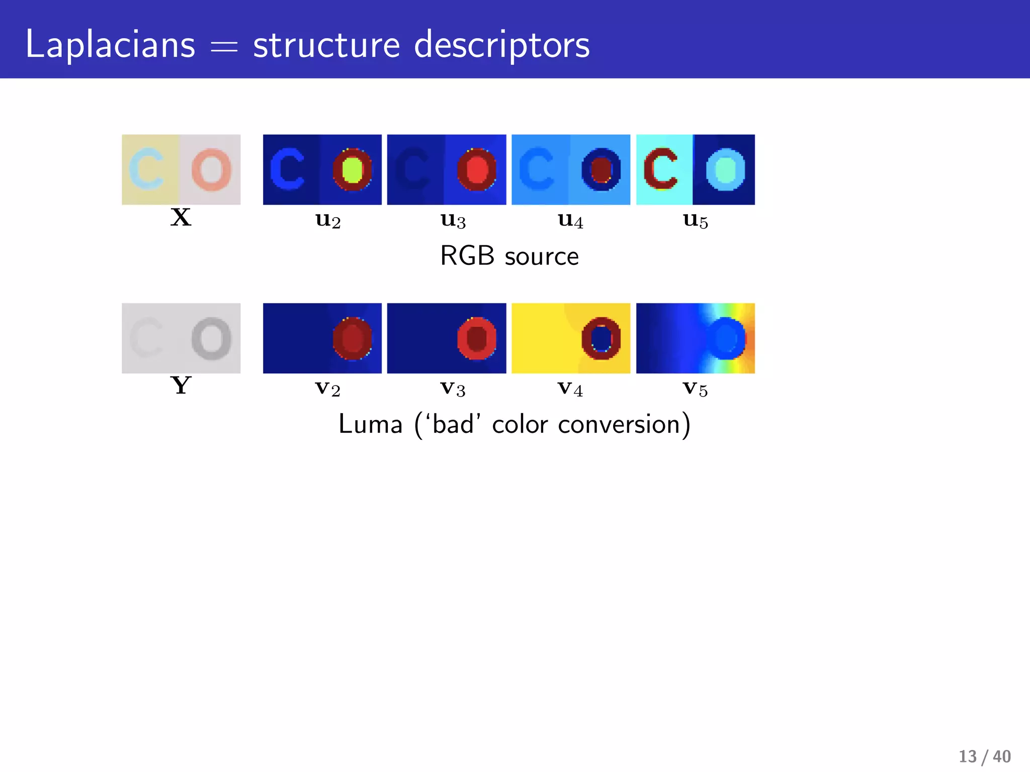
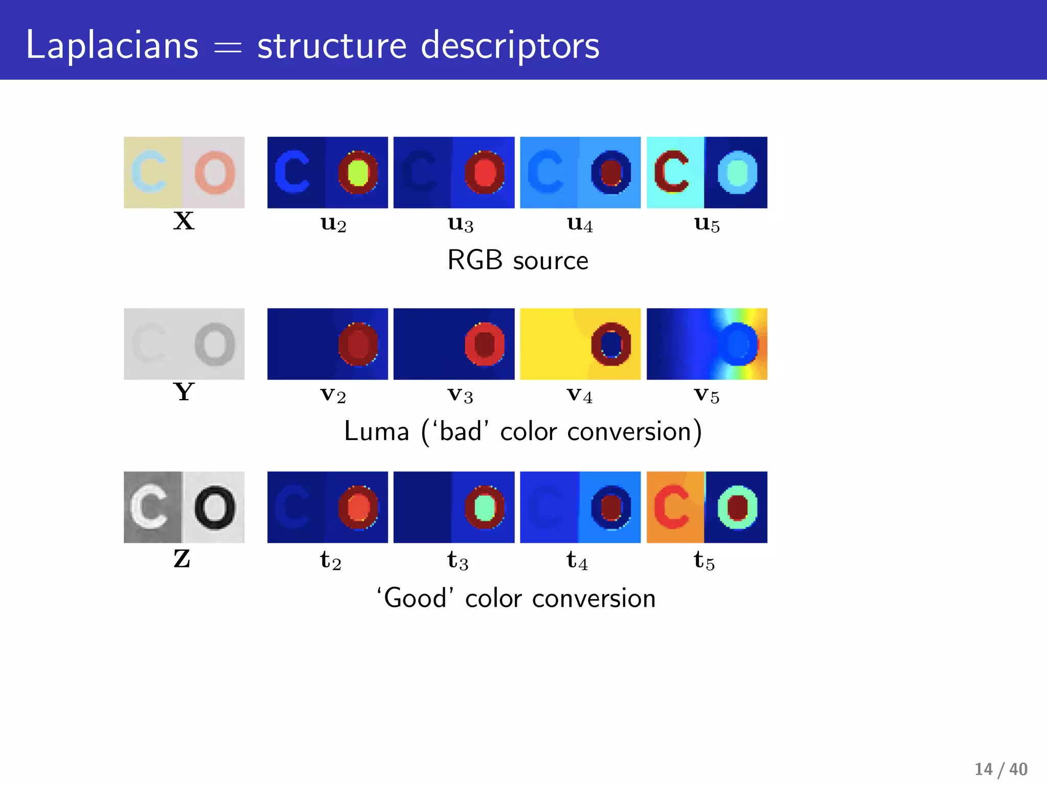
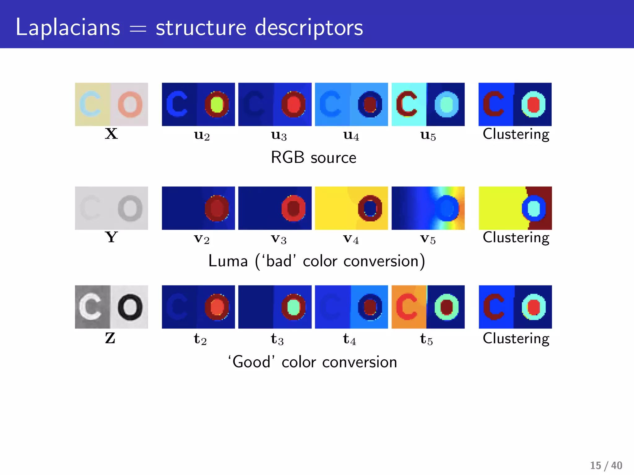
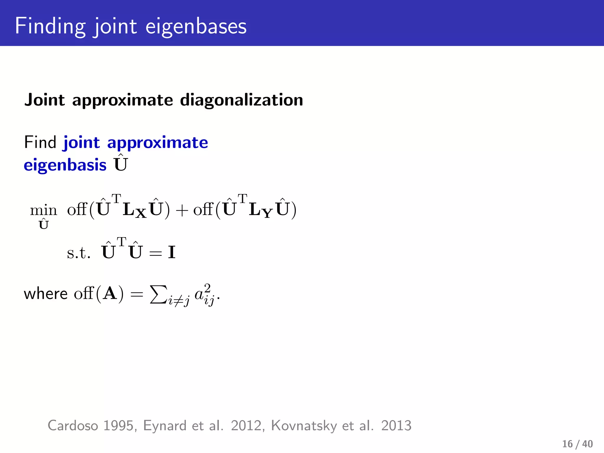
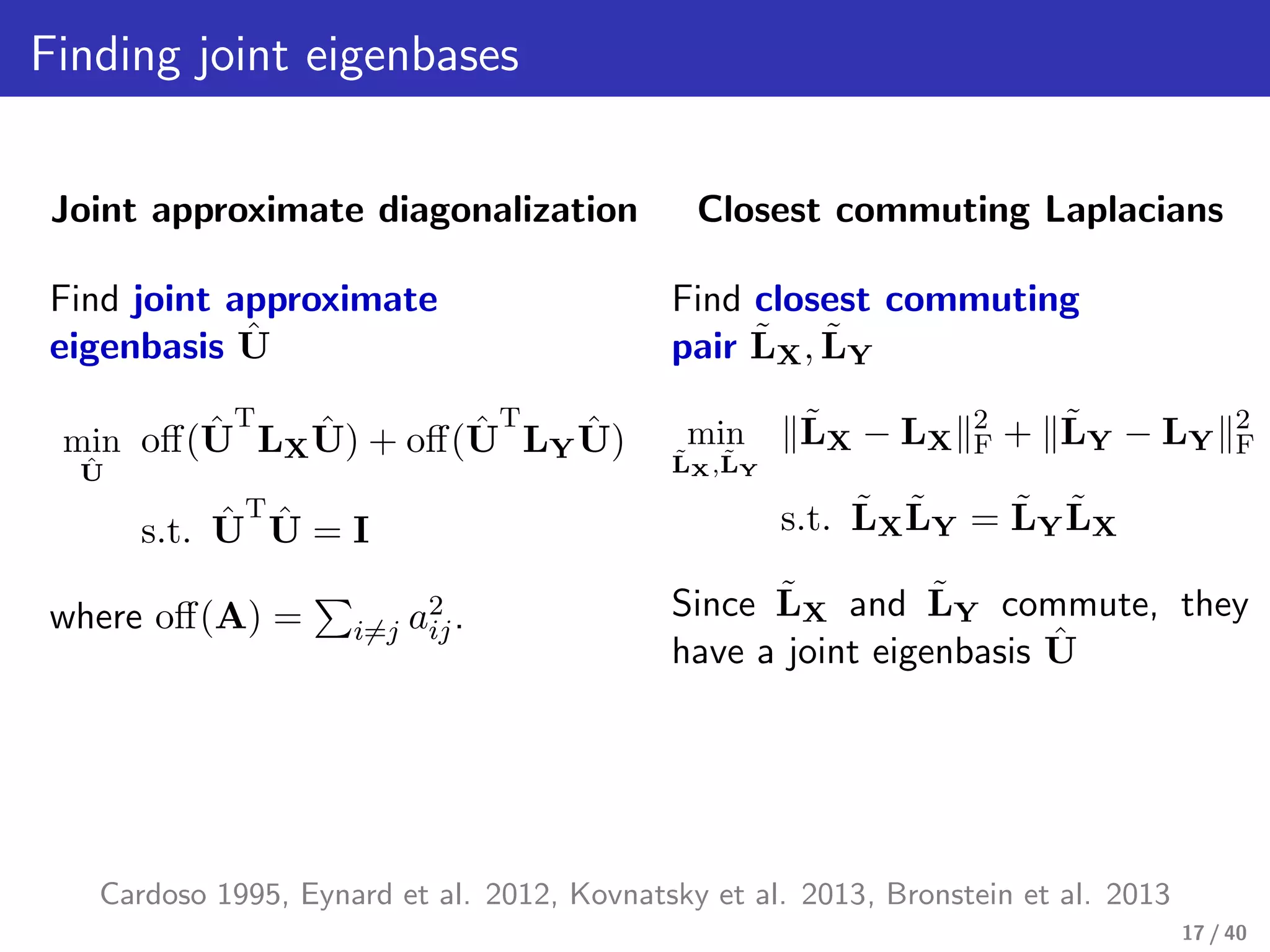
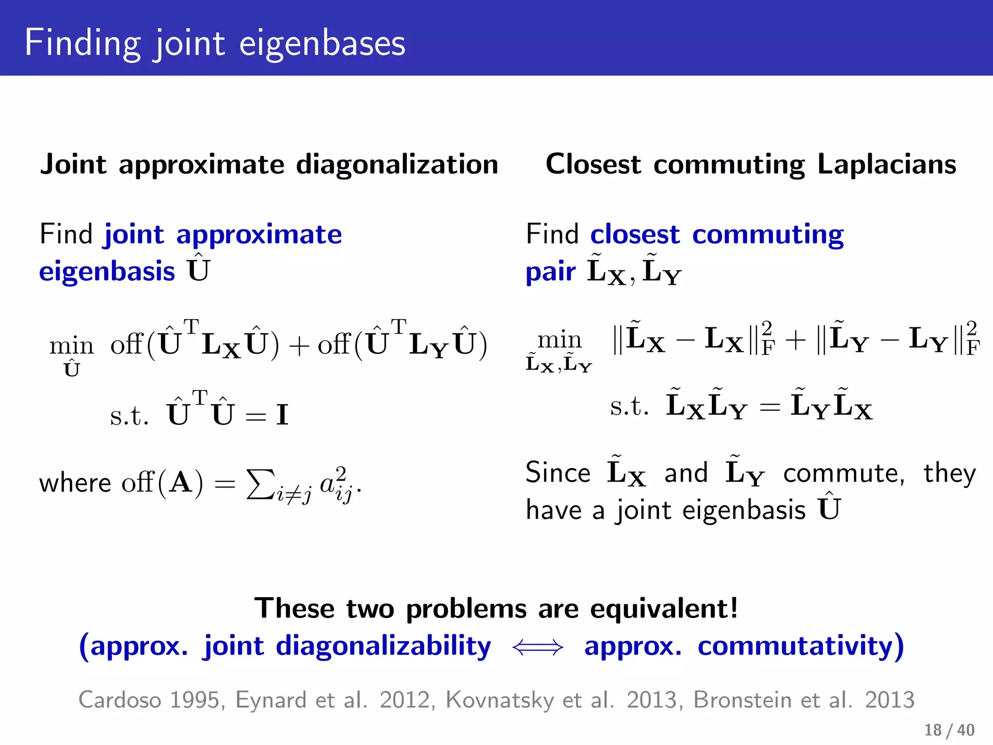
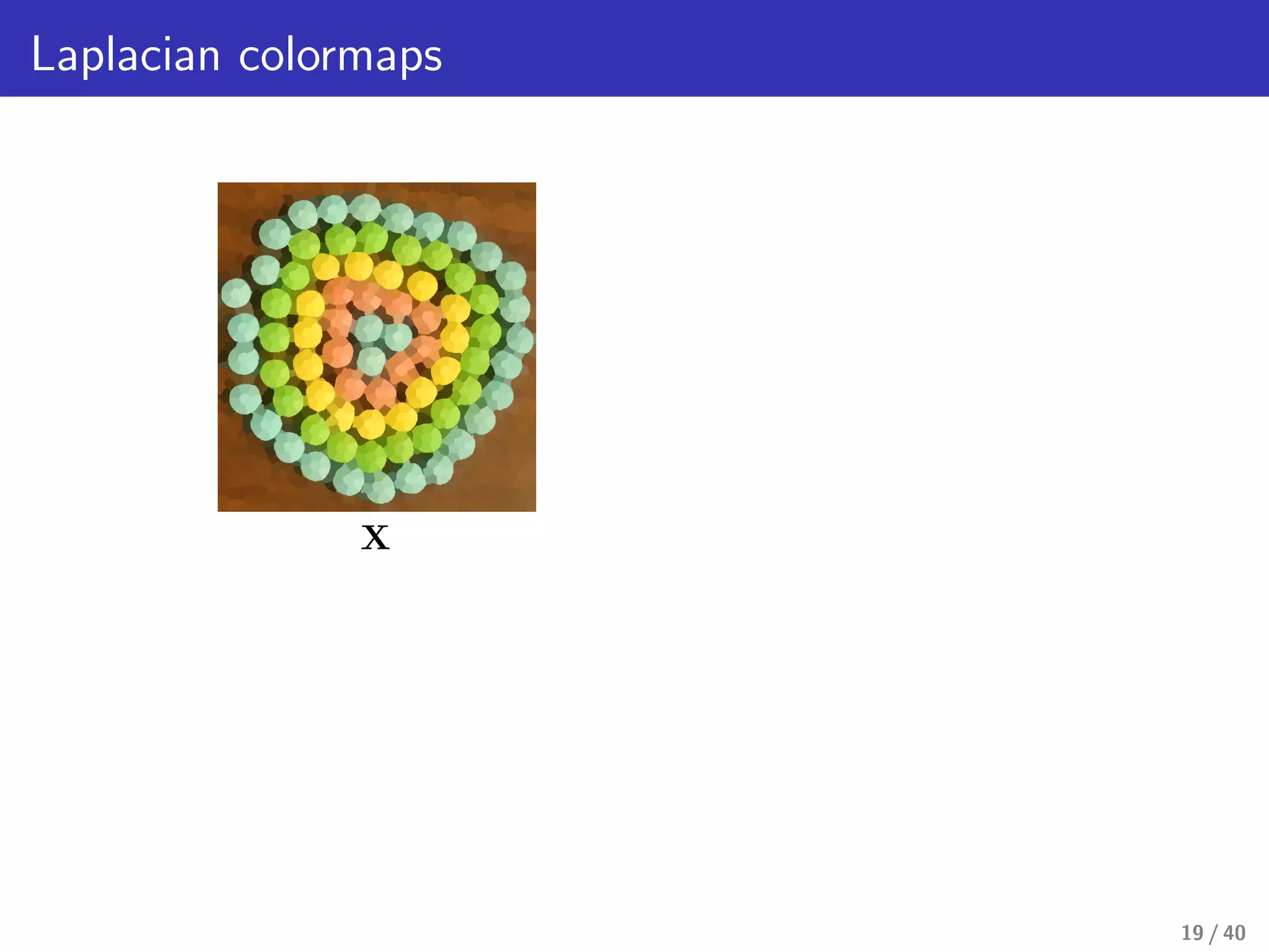
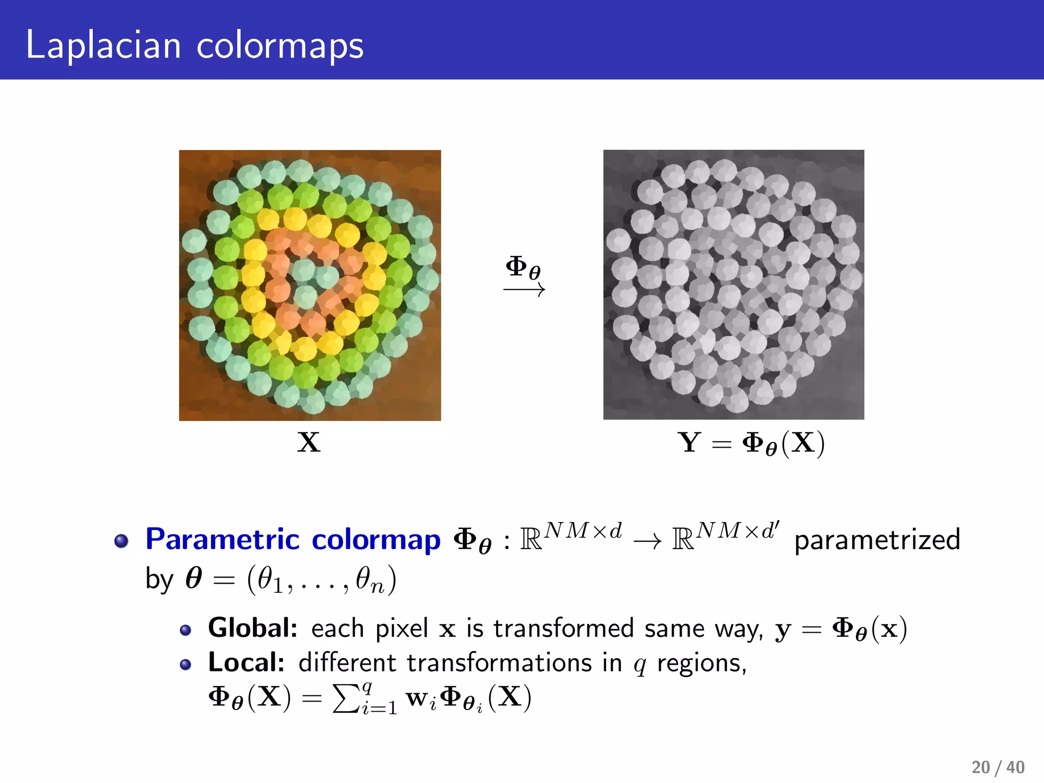
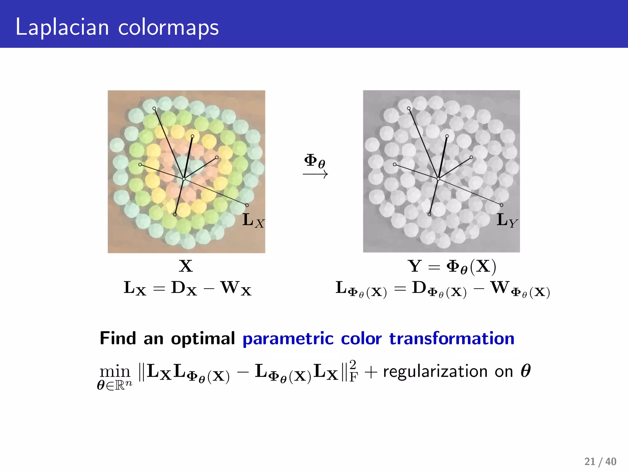
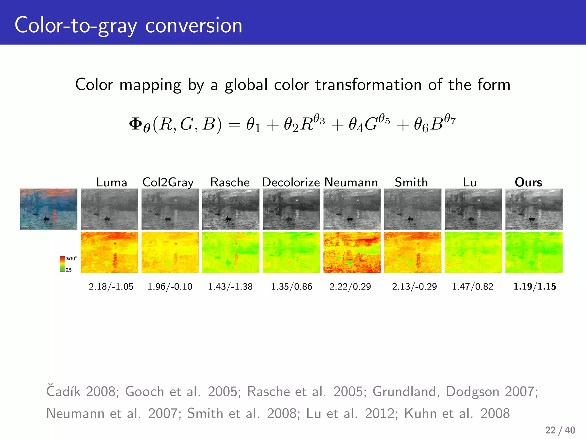
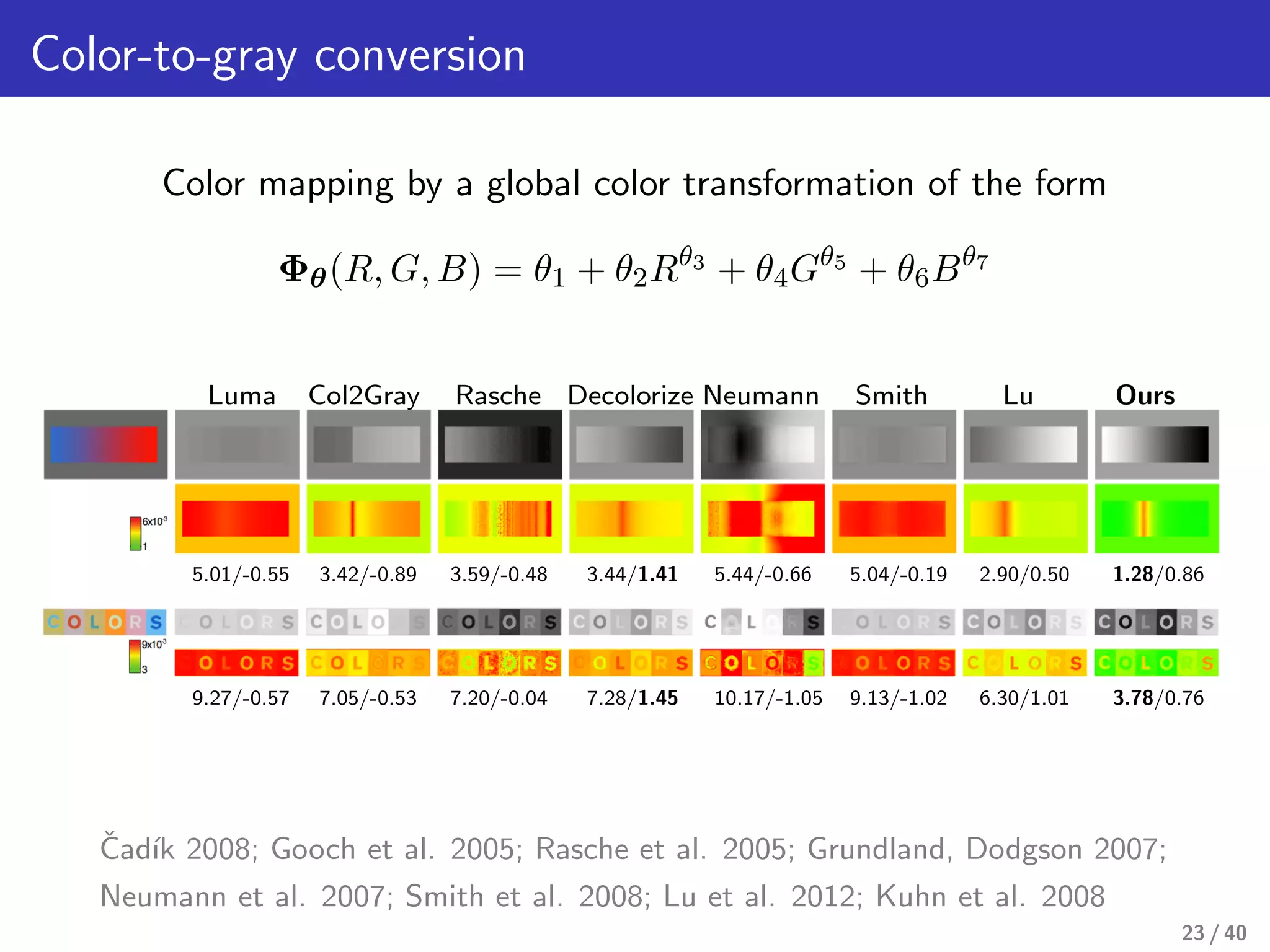
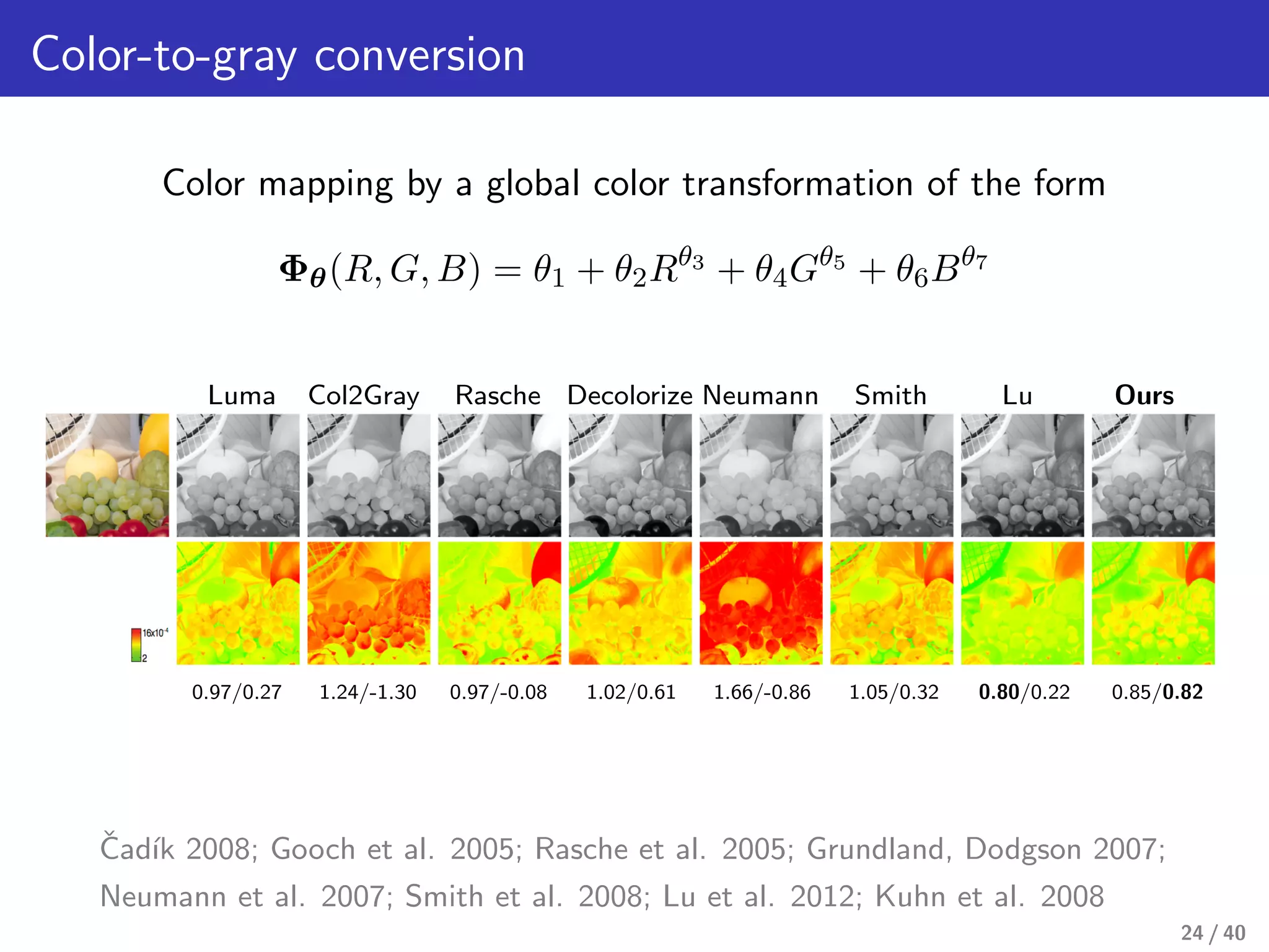
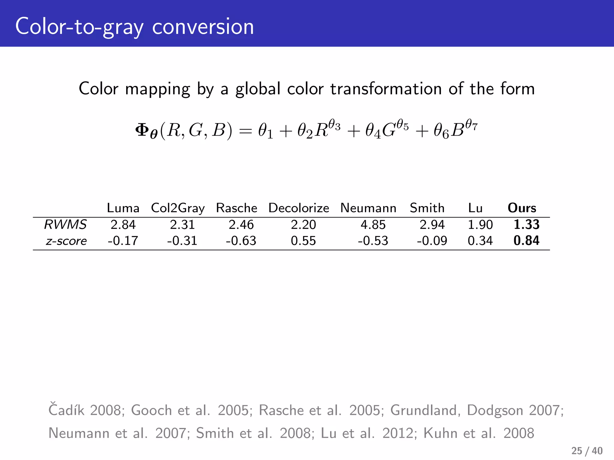
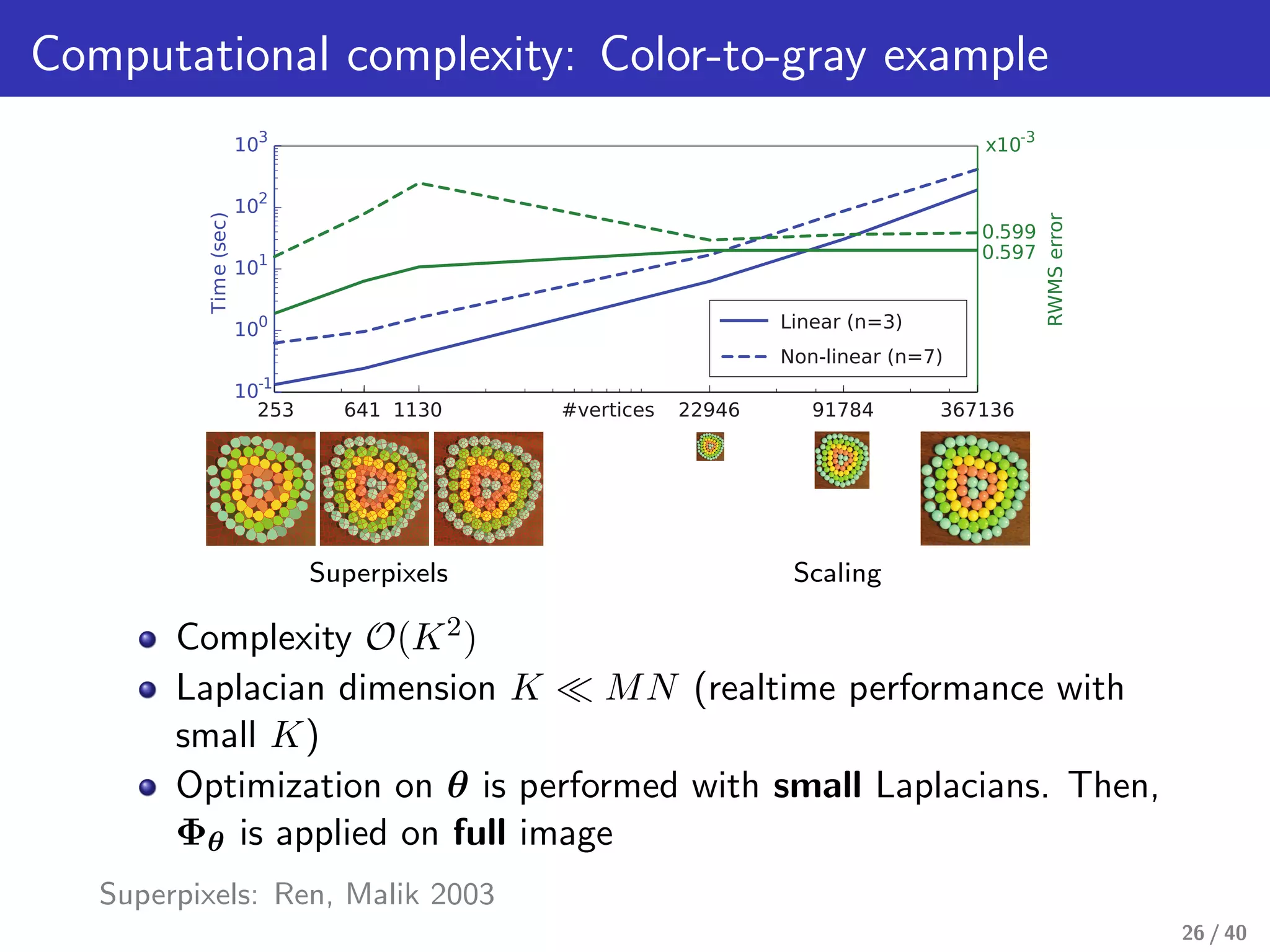
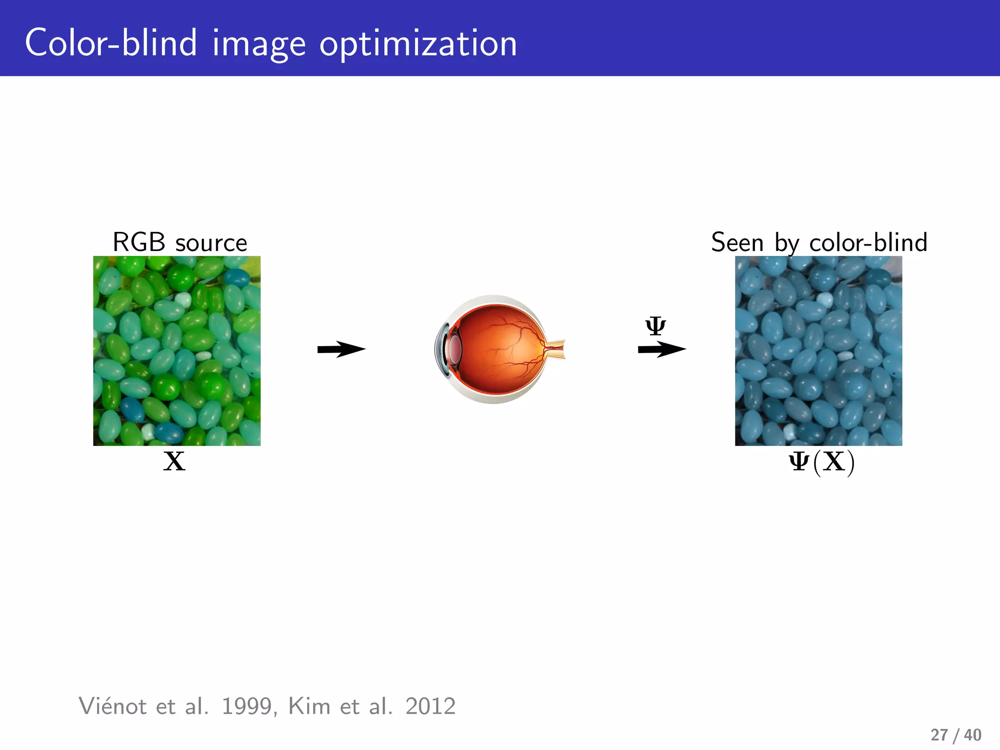
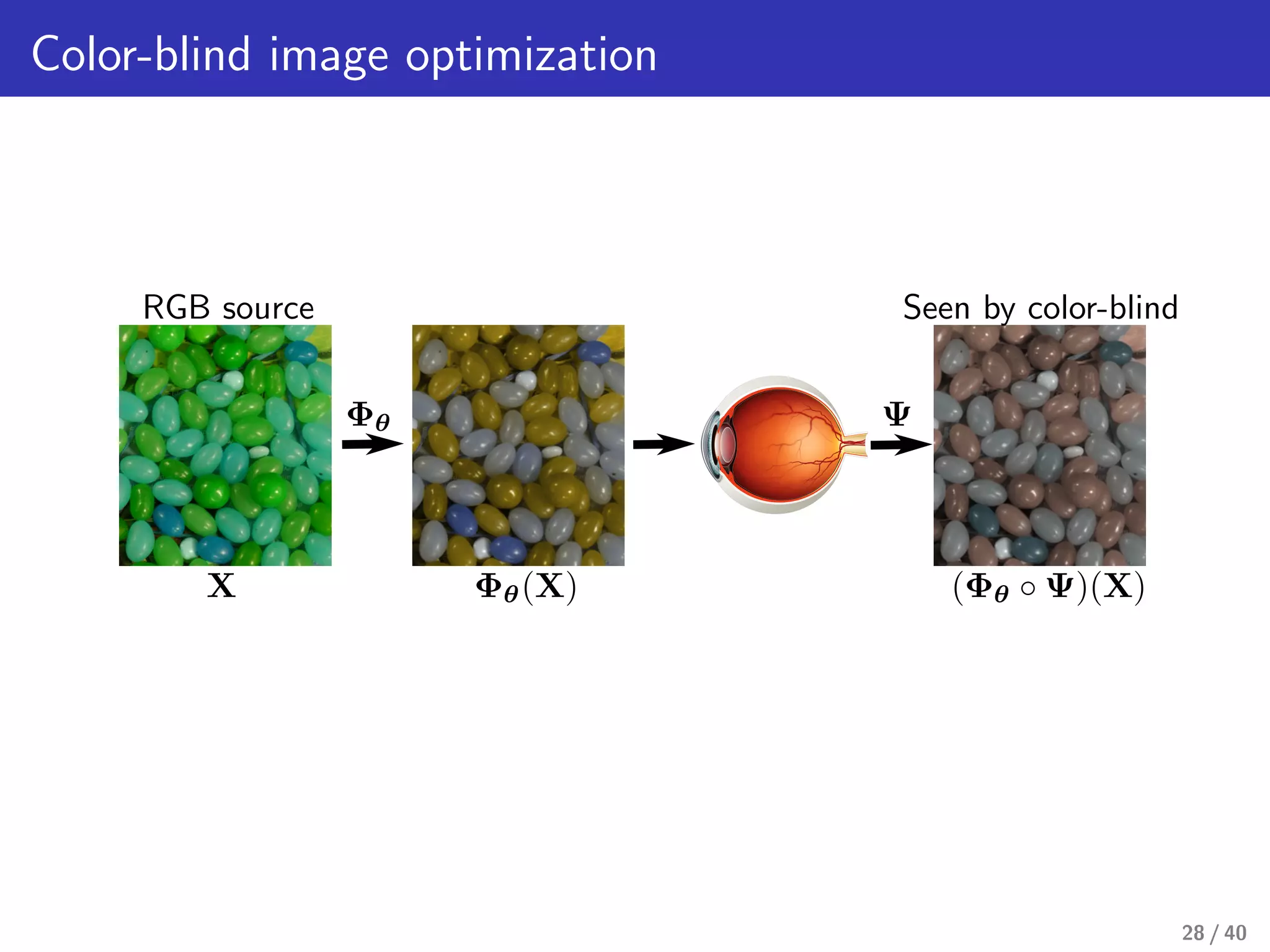
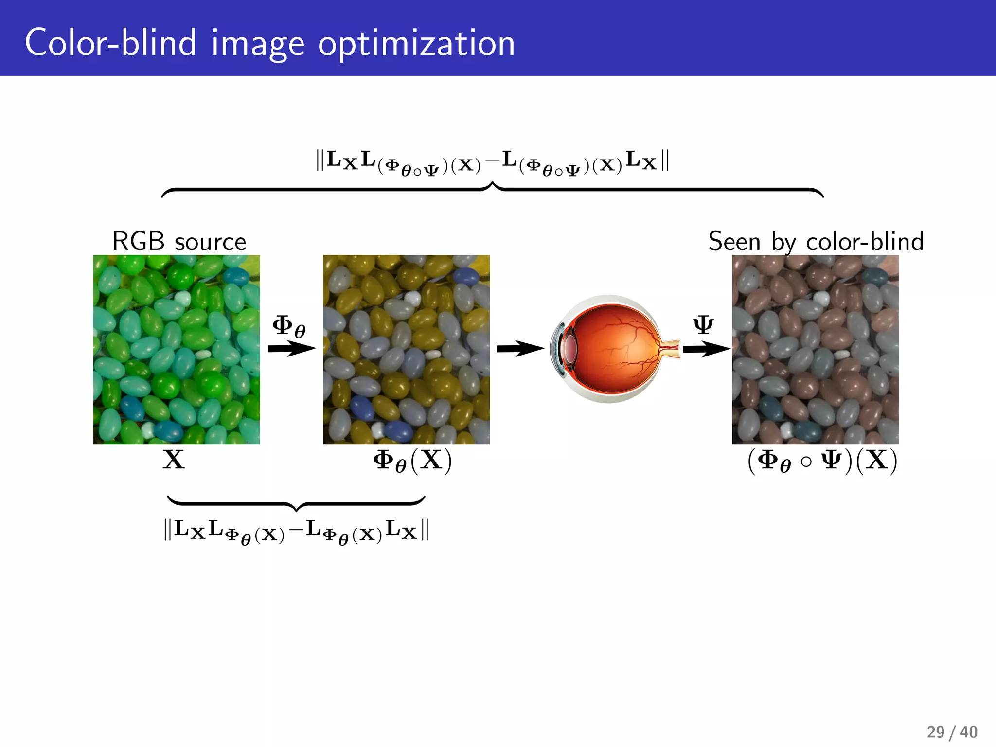
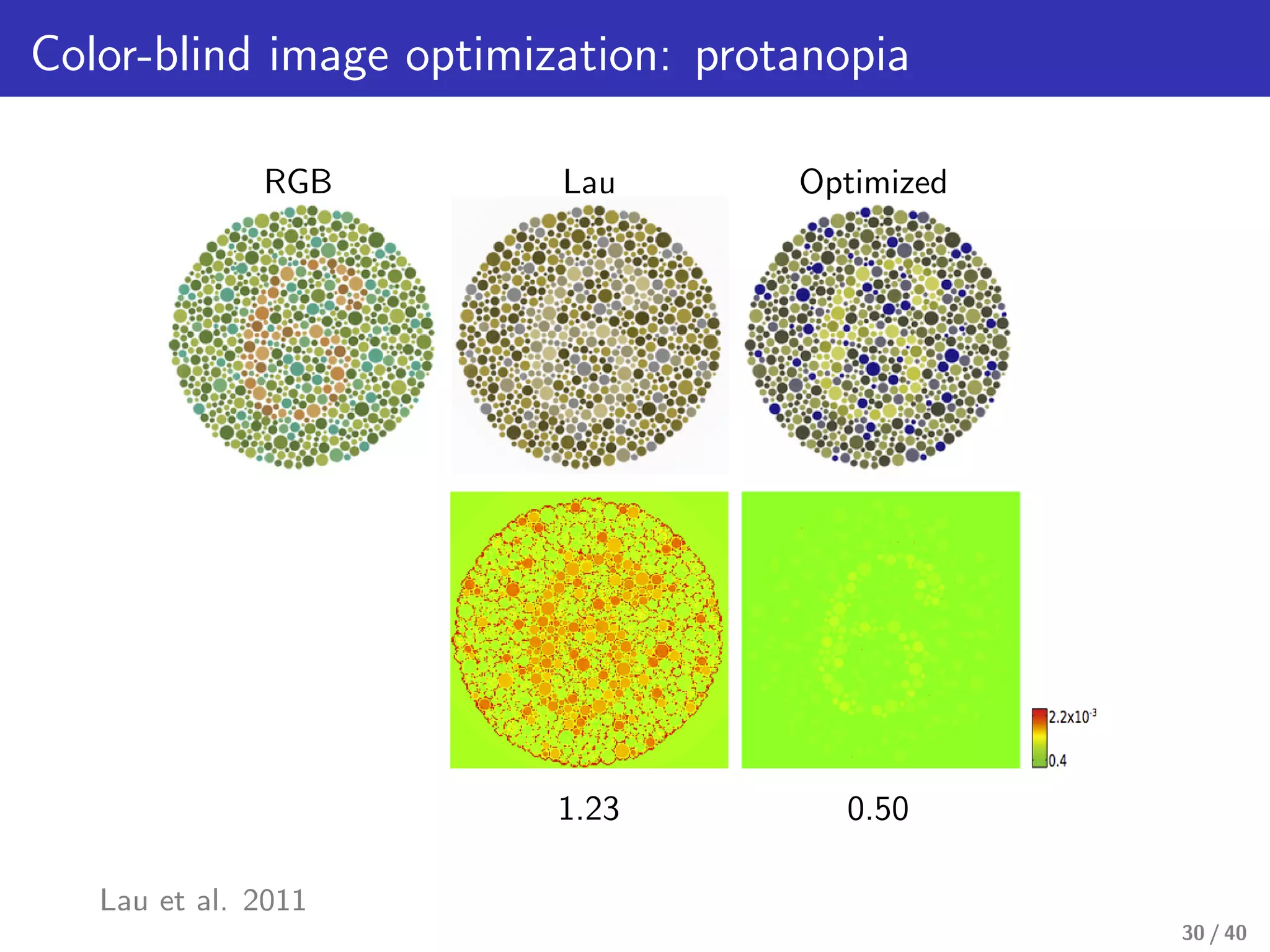
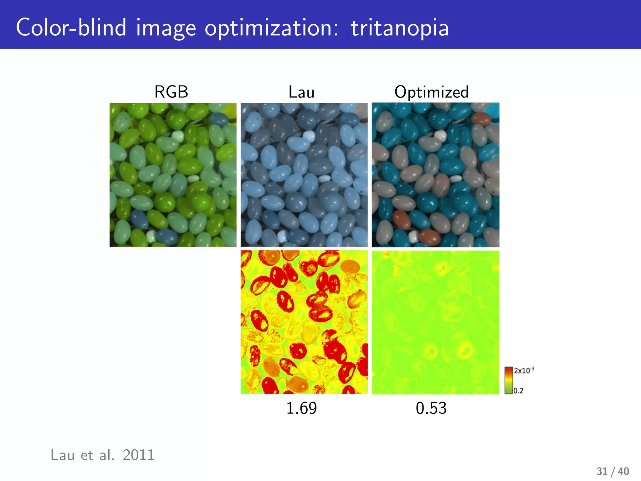
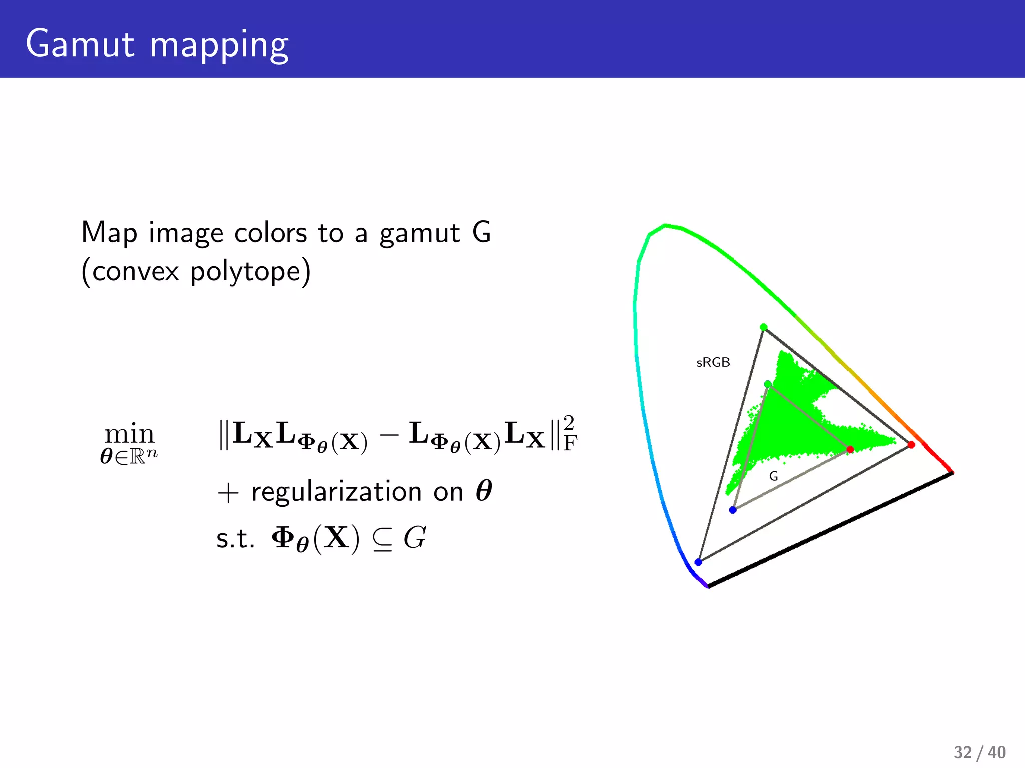
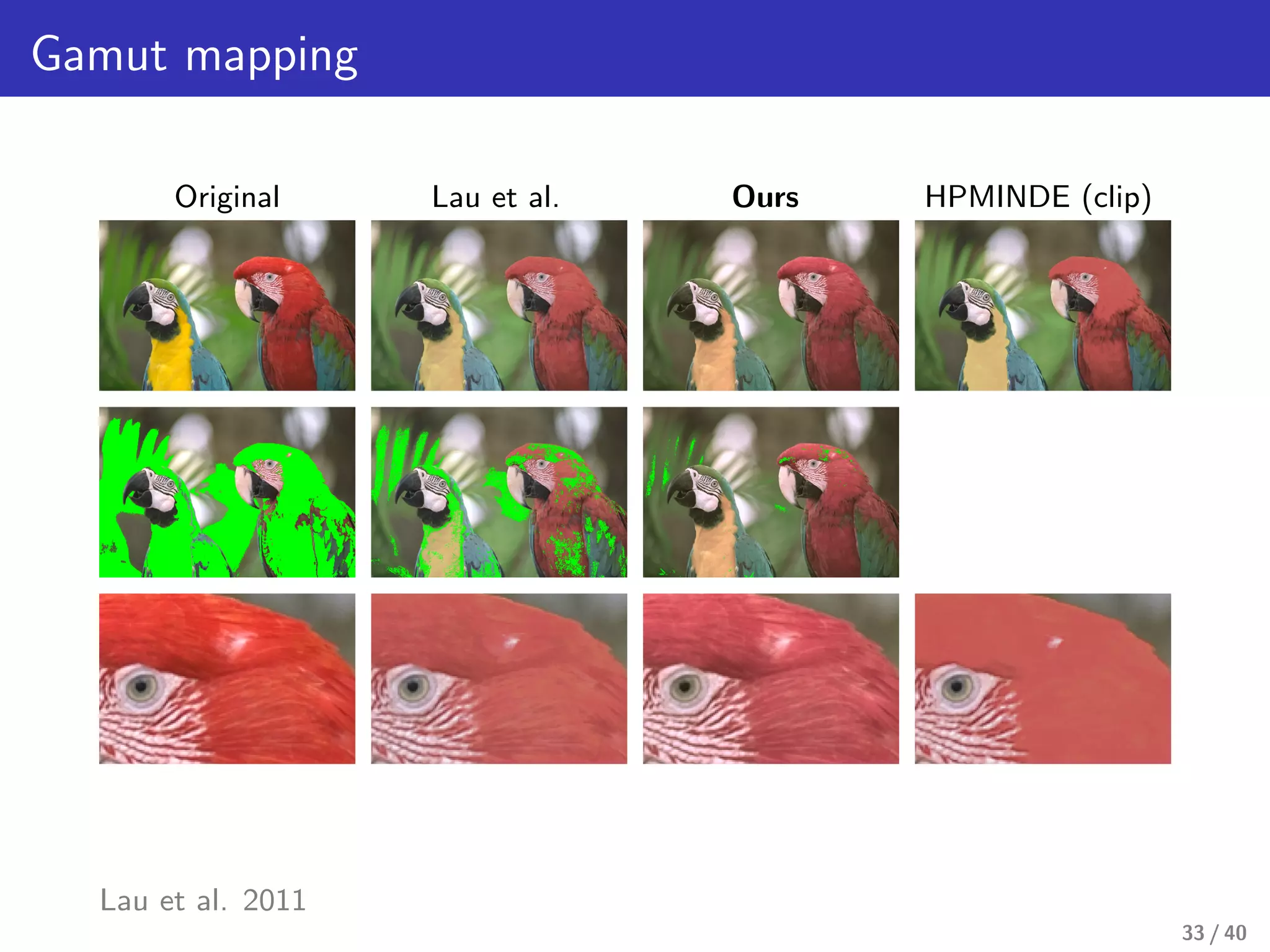
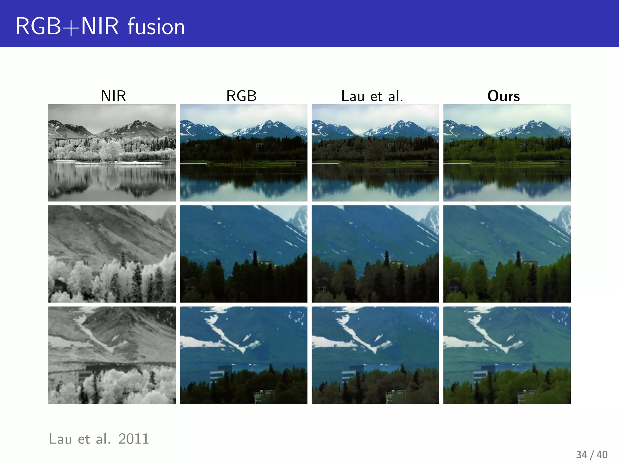
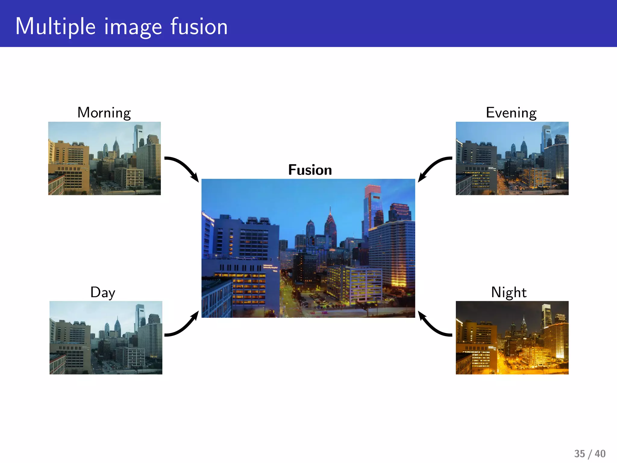
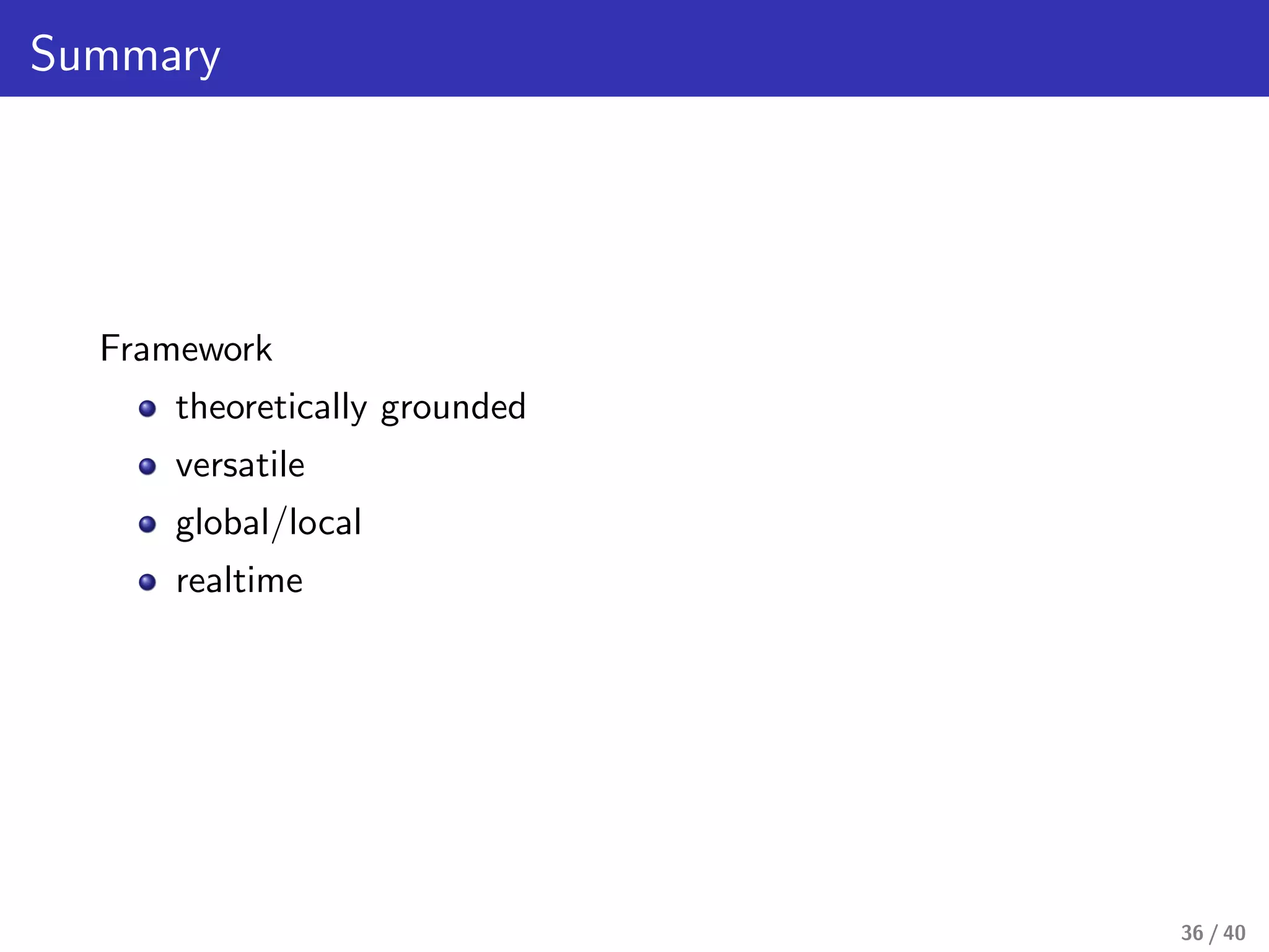
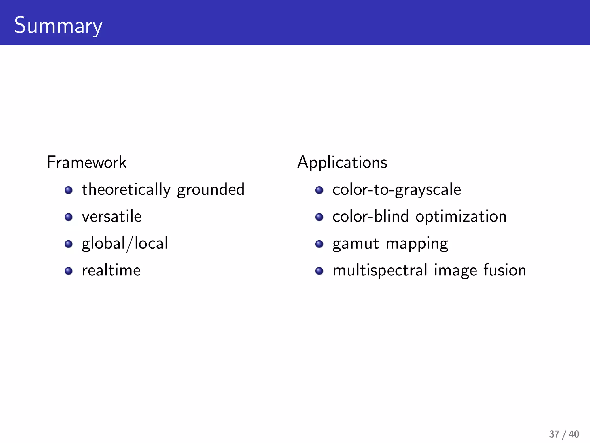
Laplacian colormaps: a framework
for structure-preserving color transformations
Davide Eynard, Artiom Kovnatsky, Michael Bronstein
Institute of Computational Science, Faculty of Informatics
University of Lugano, Switzerland
Eurographics, 8 April 2014
This research was supported by the ERC Starting Grant No. 307047 (COMET).
1 / 40
2 / 40
3 / 40
4 / 40
Color transformations
RGB source Luma
5 / 40
Color transformations
RGB source Luma
Standard color transformations may break image structure!
6 / 40
Color transformations
RGB source Luma Desired outcome
Standard color transformations may break image structure!
7 / 40
Image Laplacian
Input N × M image with d color
channels, column-stacked into an
NM × d matrix X
Represented as graph with K vertices
(e.g. superpixels) and weighted edges
8 / 40
Image Laplacian
Input N × M image with d color
channels, column-stacked into an
NM × d matrix X
Represented as graph with K vertices
(e.g. superpixels) and weighted edges
K × K adjacency matrix WX
wij = exp −
δ2
ij
2σ2
s
+
xki
− xkj
2
2
2σ2
r
K × K Laplacian
LX = DX−WX, DX = diag(
j=i
wij)
xki
xkj
wij
9 / 40
Laplacians = structure descriptors
UT
LXU = ΛX, VT
LYV = ΛY
X u4 u5 u6 u7
Y v4 v5 v6 v7
Similar structure ⇐⇒ similar Laplacian eigenvectors
10 / 40
Laplacians = structure descriptors
UT
LXU = ΛX, VT
LYV = ΛY
X u4 u5 u6 u7
Y v4 v5 v6 v7
Similar structure ⇐⇒ similar Laplacian eigenvectors
Ideally, two Laplacians are jointly diagonalizable (iff they
commute): there exists a joint eigenbasis ˆU = U = V
11 / 40
Laplacians = structure descriptors
X u2 u3 u4 u5
RGB source
12 / 40
Laplacians = structure descriptors
X u2 u3 u4 u5
RGB source
Y v2 v3 v4 v5
Luma (‘bad’ color conversion)
13 / 40
Laplacians = structure descriptors
X u2 u3 u4 u5
RGB source
Y v2 v3 v4 v5
Luma (‘bad’ color conversion)
Z t2 t3 t4 t5
‘Good’ color conversion
14 / 40
Laplacians = structure descriptors
X u2 u3 u4 u5 Clustering
RGB source
Y v2 v3 v4 v5 Clustering
Luma (‘bad’ color conversion)
Z t2 t3 t4 t5 Clustering
‘Good’ color conversion
15 / 40
Finding joint eigenbases
Joint approximate diagonalization
Find joint approximate
eigenbasis ˆU
min
ˆU
off( ˆU
T
LX
ˆU) + off( ˆU
T
LY
ˆU)
s.t. ˆU
T
ˆU = I
where off(A) = i=j a2
ij.
Cardoso 1995, Eynard et al. 2012, Kovnatsky et al. 2013
16 / 40
Finding joint eigenbases
Joint approximate diagonalization
Find joint approximate
eigenbasis ˆU
min
ˆU
off( ˆU
T
LX
ˆU) + off( ˆU
T
LY
ˆU)
s.t. ˆU
T
ˆU = I
where off(A) = i=j a2
ij.
Closest commuting Laplacians
Find closest commuting
pair ˜LX, ˜LY
min
˜LX,˜LY
˜LX − LX
2
F + ˜LY − LY
2
F
s.t. ˜LX
˜LY = ˜LY
˜LX
Since ˜LX and ˜LY commute, they
have a joint eigenbasis ˆU
Cardoso 1995, Eynard et al. 2012, Kovnatsky et al. 2013, Bronstein et al. 2013
17 / 40
Finding joint eigenbases
Joint approximate diagonalization
Find joint approximate
eigenbasis ˆU
min
ˆU
off( ˆU
T
LX
ˆU) + off( ˆU
T
LY
ˆU)
s.t. ˆU
T
ˆU = I
where off(A) = i=j a2
ij.
Closest commuting Laplacians
Find closest commuting
pair ˜LX, ˜LY
min
˜LX,˜LY
˜LX − LX
2
F + ˜LY − LY
2
F
s.t. ˜LX
˜LY = ˜LY
˜LX
Since ˜LX and ˜LY commute, they
have a joint eigenbasis ˆU
These two problems are equivalent!
(approx. joint diagonalizability ⇐⇒ approx. commutativity)
Cardoso 1995, Eynard et al. 2012, Kovnatsky et al. 2013, Bronstein et al. 2013
18 / 40
Laplacian colormaps
X
19 / 40
Laplacian colormaps
X
−→
Φθ
Y = Φθ(X)
Parametric colormap Φθ : RNM×d → RNM×d parametrized
by θ = (θ1, . . . , θn)
Global: each pixel x is transformed same way, y = Φθ(x)
Local: different transformations in q regions,
Φθ(X) =
q
i=1 wiΦθi
(X)
20 / 40
Laplacian colormaps
X
−→
Φθ
Y = Φθ(X)
LX LY
LX = DX − WX LΦθ(X) = DΦθ(X) − WΦθ(X)
Find an optimal parametric color transformation
min
θ∈Rn
LXLΦθ(X) − LΦθ(X)LX
2
F + regularization on θ
21 / 40
Color-to-gray conversion
Color mapping by a global color transformation of the form
Φθ(R, G, B) = θ1 + θ2Rθ3
+ θ4Gθ5
+ θ6Bθ7
Luma Col2Gray Rasche Decolorize Neumann Smith Lu Ours
2.18/-1.05 1.96/-0.10 1.43/-1.38 1.35/0.86 2.22/0.29 2.13/-0.29 1.47/0.82 1.19/1.15
ˇCad´ık 2008; Gooch et al. 2005; Rasche et al. 2005; Grundland, Dodgson 2007;
Neumann et al. 2007; Smith et al. 2008; Lu et al. 2012; Kuhn et al. 2008
22 / 40
Color-to-gray conversion
Color mapping by a global color transformation of the form
Φθ(R, G, B) = θ1 + θ2Rθ3
+ θ4Gθ5
+ θ6Bθ7
Luma Col2Gray Rasche Decolorize Neumann Smith Lu Ours
5.01/-0.55 3.42/-0.89 3.59/-0.48 3.44/1.41 5.44/-0.66 5.04/-0.19 2.90/0.50 1.28/0.86
9.27/-0.57 7.05/-0.53 7.20/-0.04 7.28/1.45 10.17/-1.05 9.13/-1.02 6.30/1.01 3.78/0.76
ˇCad´ık 2008; Gooch et al. 2005; Rasche et al. 2005; Grundland, Dodgson 2007;
Neumann et al. 2007; Smith et al. 2008; Lu et al. 2012; Kuhn et al. 2008
23 / 40
Color-to-gray conversion
Color mapping by a global color transformation of the form
Φθ(R, G, B) = θ1 + θ2Rθ3
+ θ4Gθ5
+ θ6Bθ7
Luma Col2Gray Rasche Decolorize Neumann Smith Lu Ours
0.97/0.27 1.24/-1.30 0.97/-0.08 1.02/0.61 1.66/-0.86 1.05/0.32 0.80/0.22 0.85/0.82
ˇCad´ık 2008; Gooch et al. 2005; Rasche et al. 2005; Grundland, Dodgson 2007;
Neumann et al. 2007; Smith et al. 2008; Lu et al. 2012; Kuhn et al. 2008
24 / 40
Color-to-gray conversion
Color mapping by a global color transformation of the form
Φθ(R, G, B) = θ1 + θ2Rθ3
+ θ4Gθ5
+ θ6Bθ7
Luma Col2Gray Rasche Decolorize Neumann Smith Lu Ours
RWMS 2.84 2.31 2.46 2.20 4.85 2.94 1.90 1.33
z-score -0.17 -0.31 -0.63 0.55 -0.53 -0.09 0.34 0.84
ˇCad´ık 2008; Gooch et al. 2005; Rasche et al. 2005; Grundland, Dodgson 2007;
Neumann et al. 2007; Smith et al. 2008; Lu et al. 2012; Kuhn et al. 2008
25 / 40
Computational complexity: Color-to-gray example
10-1
100
101
102
103
Time(sec)
#vertices253 641 1130 22946 91784 367136
0.597
RWMSerror
0.599
x10-3
Linear (n=3)
Non-linear (n=7)
Superpixels Scaling
Complexity O(K2)
Laplacian dimension K MN (realtime performance with
small K)
Optimization on θ is performed with small Laplacians. Then,
Φθ is applied on full image
Superpixels: Ren, Malik 2003
26 / 40
Color-blind image optimization
RGB source
X
Ψ
Seen by color-blind
Ψ(X)
Vi´enot et al. 1999, Kim et al. 2012
27 / 40
Color-blind image optimization
RGB source
X Φθ(X)
Ψ
Seen by color-blind
Φθ
(Φθ ◦ Ψ)(X)
28 / 40
Color-blind image optimization
RGB source
X Φθ(X)
Ψ
Seen by color-blind
Φθ
(Φθ ◦ Ψ)(X)
LXLΦθ(X)−LΦθ(X)LX
LXL(Φθ◦Ψ)(X)−L(Φθ◦Ψ)(X)LX
29 / 40
Color-blind image optimization: protanopia
RGB Lau
1.23
Optimized
0.50
Lau et al. 2011
30 / 40
Color-blind image optimization: tritanopia
RGB Lau
1.69
Optimized
0.53
Lau et al. 2011
31 / 40
Gamut mapping
Map image colors to a gamut G
(convex polytope)
min
θ∈Rn
LXLΦθ(X) − LΦθ(X)LX
2
F
+ regularization on θ
s.t. Φθ(X) ⊆ G
sRGB
G
32 / 40
Gamut mapping
Original Lau et al. Ours HPMINDE (clip)
Lau et al. 2011
33 / 40
RGB+NIR fusion
NIR RGB Lau et al. Ours
Lau et al. 2011
34 / 40
Multiple image fusion
Morning
Day
Evening
Night
Fusion
35 / 40
Summary
Framework
theoretically grounded
versatile
global/local
realtime
36 / 40
Summary
Framework
theoretically grounded
versatile
global/local
realtime
Applications
color-to-grayscale
color-blind optimization
gamut mapping
multispectral image fusion
37 / 40
Thank you!
38 / 40
Qualitative evaluation
Web survey
124 volunteers, 2884 pairwise evaluations
Thurstone’s law of comparative judgements → z-score
Consistent with ˇCad´ık’s results
39 / 40
Extension: local colormap
RGB Luma Lau et al.
Global Local Clusters
Φθ(X) = q
i=1 wiΦθi
(X)
Lau et al. 2011
40 / 40

Laplacian Colormaps: a framework for structure-preserving color transformations

  • 1.
    Laplacian colormaps: aframework for structure-preserving color transformations Davide Eynard, Artiom Kovnatsky, Michael Bronstein Institute of Computational Science, Faculty of Informatics University of Lugano, Switzerland Eurographics, 8 April 2014 This research was supported by the ERC Starting Grant No. 307047 (COMET). 1 / 40
  • 2.
  • 3.
  • 4.
  • 5.
  • 6.
    Color transformations RGB sourceLuma Standard color transformations may break image structure! 6 / 40
  • 7.
    Color transformations RGB sourceLuma Desired outcome Standard color transformations may break image structure! 7 / 40
  • 8.
    Image Laplacian Input N× M image with d color channels, column-stacked into an NM × d matrix X Represented as graph with K vertices (e.g. superpixels) and weighted edges 8 / 40
  • 9.
    Image Laplacian Input N× M image with d color channels, column-stacked into an NM × d matrix X Represented as graph with K vertices (e.g. superpixels) and weighted edges K × K adjacency matrix WX wij = exp − δ2 ij 2σ2 s + xki − xkj 2 2 2σ2 r K × K Laplacian LX = DX−WX, DX = diag( j=i wij) xki xkj wij 9 / 40
  • 10.
    Laplacians = structuredescriptors UT LXU = ΛX, VT LYV = ΛY X u4 u5 u6 u7 Y v4 v5 v6 v7 Similar structure ⇐⇒ similar Laplacian eigenvectors 10 / 40
  • 11.
    Laplacians = structuredescriptors UT LXU = ΛX, VT LYV = ΛY X u4 u5 u6 u7 Y v4 v5 v6 v7 Similar structure ⇐⇒ similar Laplacian eigenvectors Ideally, two Laplacians are jointly diagonalizable (iff they commute): there exists a joint eigenbasis ˆU = U = V 11 / 40
  • 12.
    Laplacians = structuredescriptors X u2 u3 u4 u5 RGB source 12 / 40
  • 13.
    Laplacians = structuredescriptors X u2 u3 u4 u5 RGB source Y v2 v3 v4 v5 Luma (‘bad’ color conversion) 13 / 40
  • 14.
    Laplacians = structuredescriptors X u2 u3 u4 u5 RGB source Y v2 v3 v4 v5 Luma (‘bad’ color conversion) Z t2 t3 t4 t5 ‘Good’ color conversion 14 / 40
  • 15.
    Laplacians = structuredescriptors X u2 u3 u4 u5 Clustering RGB source Y v2 v3 v4 v5 Clustering Luma (‘bad’ color conversion) Z t2 t3 t4 t5 Clustering ‘Good’ color conversion 15 / 40
  • 16.
    Finding joint eigenbases Jointapproximate diagonalization Find joint approximate eigenbasis ˆU min ˆU off( ˆU T LX ˆU) + off( ˆU T LY ˆU) s.t. ˆU T ˆU = I where off(A) = i=j a2 ij. Cardoso 1995, Eynard et al. 2012, Kovnatsky et al. 2013 16 / 40
  • 17.
    Finding joint eigenbases Jointapproximate diagonalization Find joint approximate eigenbasis ˆU min ˆU off( ˆU T LX ˆU) + off( ˆU T LY ˆU) s.t. ˆU T ˆU = I where off(A) = i=j a2 ij. Closest commuting Laplacians Find closest commuting pair ˜LX, ˜LY min ˜LX,˜LY ˜LX − LX 2 F + ˜LY − LY 2 F s.t. ˜LX ˜LY = ˜LY ˜LX Since ˜LX and ˜LY commute, they have a joint eigenbasis ˆU Cardoso 1995, Eynard et al. 2012, Kovnatsky et al. 2013, Bronstein et al. 2013 17 / 40
  • 18.
    Finding joint eigenbases Jointapproximate diagonalization Find joint approximate eigenbasis ˆU min ˆU off( ˆU T LX ˆU) + off( ˆU T LY ˆU) s.t. ˆU T ˆU = I where off(A) = i=j a2 ij. Closest commuting Laplacians Find closest commuting pair ˜LX, ˜LY min ˜LX,˜LY ˜LX − LX 2 F + ˜LY − LY 2 F s.t. ˜LX ˜LY = ˜LY ˜LX Since ˜LX and ˜LY commute, they have a joint eigenbasis ˆU These two problems are equivalent! (approx. joint diagonalizability ⇐⇒ approx. commutativity) Cardoso 1995, Eynard et al. 2012, Kovnatsky et al. 2013, Bronstein et al. 2013 18 / 40
  • 19.
  • 20.
    Laplacian colormaps X −→ Φθ Y =Φθ(X) Parametric colormap Φθ : RNM×d → RNM×d parametrized by θ = (θ1, . . . , θn) Global: each pixel x is transformed same way, y = Φθ(x) Local: different transformations in q regions, Φθ(X) = q i=1 wiΦθi (X) 20 / 40
  • 21.
    Laplacian colormaps X −→ Φθ Y =Φθ(X) LX LY LX = DX − WX LΦθ(X) = DΦθ(X) − WΦθ(X) Find an optimal parametric color transformation min θ∈Rn LXLΦθ(X) − LΦθ(X)LX 2 F + regularization on θ 21 / 40
  • 22.
    Color-to-gray conversion Color mappingby a global color transformation of the form Φθ(R, G, B) = θ1 + θ2Rθ3 + θ4Gθ5 + θ6Bθ7 Luma Col2Gray Rasche Decolorize Neumann Smith Lu Ours 2.18/-1.05 1.96/-0.10 1.43/-1.38 1.35/0.86 2.22/0.29 2.13/-0.29 1.47/0.82 1.19/1.15 ˇCad´ık 2008; Gooch et al. 2005; Rasche et al. 2005; Grundland, Dodgson 2007; Neumann et al. 2007; Smith et al. 2008; Lu et al. 2012; Kuhn et al. 2008 22 / 40
  • 23.
    Color-to-gray conversion Color mappingby a global color transformation of the form Φθ(R, G, B) = θ1 + θ2Rθ3 + θ4Gθ5 + θ6Bθ7 Luma Col2Gray Rasche Decolorize Neumann Smith Lu Ours 5.01/-0.55 3.42/-0.89 3.59/-0.48 3.44/1.41 5.44/-0.66 5.04/-0.19 2.90/0.50 1.28/0.86 9.27/-0.57 7.05/-0.53 7.20/-0.04 7.28/1.45 10.17/-1.05 9.13/-1.02 6.30/1.01 3.78/0.76 ˇCad´ık 2008; Gooch et al. 2005; Rasche et al. 2005; Grundland, Dodgson 2007; Neumann et al. 2007; Smith et al. 2008; Lu et al. 2012; Kuhn et al. 2008 23 / 40
  • 24.
    Color-to-gray conversion Color mappingby a global color transformation of the form Φθ(R, G, B) = θ1 + θ2Rθ3 + θ4Gθ5 + θ6Bθ7 Luma Col2Gray Rasche Decolorize Neumann Smith Lu Ours 0.97/0.27 1.24/-1.30 0.97/-0.08 1.02/0.61 1.66/-0.86 1.05/0.32 0.80/0.22 0.85/0.82 ˇCad´ık 2008; Gooch et al. 2005; Rasche et al. 2005; Grundland, Dodgson 2007; Neumann et al. 2007; Smith et al. 2008; Lu et al. 2012; Kuhn et al. 2008 24 / 40
  • 25.
    Color-to-gray conversion Color mappingby a global color transformation of the form Φθ(R, G, B) = θ1 + θ2Rθ3 + θ4Gθ5 + θ6Bθ7 Luma Col2Gray Rasche Decolorize Neumann Smith Lu Ours RWMS 2.84 2.31 2.46 2.20 4.85 2.94 1.90 1.33 z-score -0.17 -0.31 -0.63 0.55 -0.53 -0.09 0.34 0.84 ˇCad´ık 2008; Gooch et al. 2005; Rasche et al. 2005; Grundland, Dodgson 2007; Neumann et al. 2007; Smith et al. 2008; Lu et al. 2012; Kuhn et al. 2008 25 / 40
  • 26.
    Computational complexity: Color-to-grayexample 10-1 100 101 102 103 Time(sec) #vertices253 641 1130 22946 91784 367136 0.597 RWMSerror 0.599 x10⁻³ Linear (n=3) Non-linear (n=7) Superpixels Scaling Complexity O(K2) Laplacian dimension K MN (realtime performance with small K) Optimization on θ is performed with small Laplacians. Then, Φθ is applied on full image Superpixels: Ren, Malik 2003 26 / 40
  • 27.
    Color-blind image optimization RGBsource X Ψ Seen by color-blind Ψ(X) Vi´enot et al. 1999, Kim et al. 2012 27 / 40
  • 28.
    Color-blind image optimization RGBsource X Φθ(X) Ψ Seen by color-blind Φθ (Φθ ◦ Ψ)(X) 28 / 40
  • 29.
    Color-blind image optimization RGBsource X Φθ(X) Ψ Seen by color-blind Φθ (Φθ ◦ Ψ)(X) LXLΦθ(X)−LΦθ(X)LX LXL(Φθ◦Ψ)(X)−L(Φθ◦Ψ)(X)LX 29 / 40
  • 30.
    Color-blind image optimization:protanopia RGB Lau 1.23 Optimized 0.50 Lau et al. 2011 30 / 40
  • 31.
    Color-blind image optimization:tritanopia RGB Lau 1.69 Optimized 0.53 Lau et al. 2011 31 / 40
  • 32.
    Gamut mapping Map imagecolors to a gamut G (convex polytope) min θ∈Rn LXLΦθ(X) − LΦθ(X)LX 2 F + regularization on θ s.t. Φθ(X) ⊆ G sRGB G 32 / 40
  • 33.
    Gamut mapping Original Lauet al. Ours HPMINDE (clip) Lau et al. 2011 33 / 40
  • 34.
    RGB+NIR fusion NIR RGBLau et al. Ours Lau et al. 2011 34 / 40
  • 35.
  • 36.
  • 37.
  • 38.
  • 39.
    Qualitative evaluation Web survey 124volunteers, 2884 pairwise evaluations Thurstone’s law of comparative judgements → z-score Consistent with ˇCad´ık’s results 39 / 40
  • 40.
    Extension: local colormap RGBLuma Lau et al. Global Local Clusters Φθ(X) = q i=1 wiΦθi (X) Lau et al. 2011 40 / 40