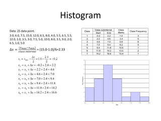
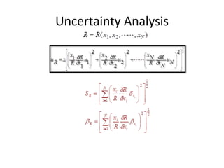
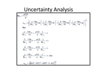
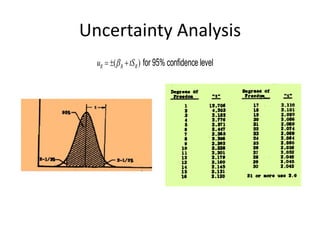
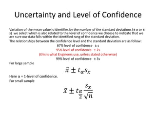
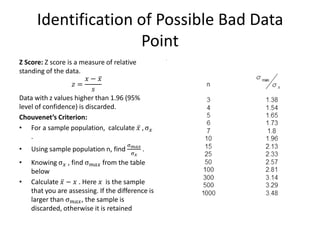
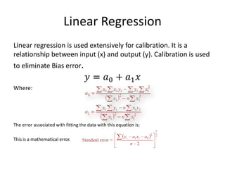
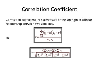
Statistics: Terms and Definitions 
Population: All data, continuous 
Sample: A subset of data, discrete. Use sample for inferential statistics. 
Every statistical problem contains five elements: 
•Questions to be answered. Identification of the populations 
•Design of experiment, sampling procedure 
•Analysis of the sampled data (equations and distributions) 
•Inference (based on confidence level) 
•How good the inference is, measure of goodness
Statistics: Terms and Definitions 
Measurements: Single Point 
Multiple Point 
Uncertainty is total error associated with measurements with specific level of confidence. 
Errors: Bias or fixed error (Systematic Error) 
Precision or random error 
Mean = 휇=푥 = 푥푖 푛 , 푥푖 is the sample and n is the total number of the samples. 
Variance = 휎2=푠2= 1 푛−1 (푥 −푥푖)2 
Average deviation from the mean= 1 푛 (푥 −푥푖)2 
R.M.S. Deviation from the mean = 1 푛 (푥 −푥푖)2 
Standard Deviation (SD)=푠=휎= 푠2=휎2 
Coefficient of Variation: It is a relative variation of the data, 푠 푥 
Standard Error of the Mean = 푠푥 = 푠 푛 
Mode: The most frequent items in the measurement 
Median: Central item when the data is arranged in ascending or descending order. 
Degrees of freedom: F or DF = n-K . Here k is the number of constraints imposed on the data.
Probability Density Function (PDF) 
Probability is a measure of occurrence 
Probability of an event between a & b 
P(a<x<b) = 푝푥푑푥 푏 푎 
Total Probability = 푝푥푑푥 ∞ −∞ 
Gaussian Distribution 
푝푥 1 휎푥2휋 푒 − 12(휎푥)2푥−휇2
Standard Normal Distribution 
If the data is large and random, then with the following conversion, it should follow a standard normal distribution. 
푧= 푥−휇 휎푥 
푝푧 12휋 푒− 푧22 
Area under the curve is one.
Histogram 
Histogram provides the probability of events within each increment. Histogram can be used to check if the data follows a standard distribution or not. The following steps can be used to draw a histogram: 
–Choose a number of class intervals (usually between 5 and 20) that covers the data range. Select the class marks which are the mid-point of the class intervals. If you arrange data in ascending order, the first data should fall in the first class interval. 
–For each class interval, determine the number of data that fall within that interval. If a data falls exactly at the division point, then it is placed in the lower interval. 
–Construct rectangles with centers at the class marks and areas proportional to class frequencies. If the widths of the rectangles are the same, then the height of the rectangles represent the class frequencies.
Histogram 
Data: 25 data point. 
3.0, 6.0, 7.5, 15.0, 12.0, 6.5, 8.0, 4.0, 5.5, 6.5, 5.5, 
12.0, 1.0, 3.5, 3.0, 7.5, 5.0, 10.0, 8.0, 3.5, 9.0, 2.0, 
6.5, 1.0, 5.0 
Δ푥 = 
(푥푚푎푥−푥푚푖푛) 
푐푙푎푠푠 푖푛푡푒푟푣푎푙 
= (15.0-1.0)/6=2.33 
0.2 2.4 2.2 2 1 x  x  x     
2.2 2.4 4.6 3 2 x  x  x    
4.6 2.4 7.0 4 3 x  x  x    
7.0 2.4 9.4 5 4 x  x  x    
9.4 2.4 11.8 6 5 x  x  x    
11.8 2.4 14.2 7 6 x  x  x    
14.2 2.4 16.6 8 7 x  x  x    
Class 
Class subinterval Class 
Marks 
Class Frequency 
Start End 
1 -0.2 2.2 1.0 3 
2 2.2 4.6 3.4 5 
3 4.6 7.0 5.8 8 
4 7.0 9.4 8.2 5 
5 9.4 11.8 10.6 1 
6 11.8 14.2 13.0 2 
7 14.2 16.6 15.4 1
Uncertainty Analysis
Uncertainty Analysis utSRRR() for 95% confidence level
Uncertainty and Level of Confidence 
Variation of the mean value is identifies by the number of the standard deviations (± σ or ± s) we select which is also related to the level of confidence we choose to indicate that we are sure our data falls within the identified rang of the standard deviation. 
The relationships between the confidence level and the standard deviation are as follow: 
67% level of confidence ± s 
95% level of confidence ± 2s 
(this is what Engineers use, unless stated otherwise) 
99% level of confidence ± 3s 
For large sample 푥 ±푡훼푠푥 
Here α = 1-level of confidence. 
For small sample 푥 ±푡훼 2 푠푥 푛
Identification of Possible Bad Data Point 
Z Score: Z score is a measure of relative standing of the data. 
푧= 푥−푥 푠 
Data with z values higher than 1.96 (95% level of confidence) is discarded. 
Chouvenet’s Criterion: 
•For a sample population, calculate 푥 ,σ푥 . 
•Using sample population n, find σ푚푎푥 σ푥 . 
•Knowing σ푥 , find σ푚푎푥 from the table below 
•Calculate 푥 −푥 . Here 푥 is the sample that you are assessing. If the difference is larger than σ푚푎푥, the sample is discarded, otherwise it is retained 
.
Linear Regression 
Linear regression is used extensively for calibration. It is a relationship between input (x) and output (y). Calibration is used to eliminate Bias error. 
푦=푎0+푎1푥 
Where: 
The error associated with fitting the data with this equation is: 
This is a mathematical error.
Correlation Coefficient 
Correlation coefficient (r) is a measure of the strength of a linear relationship between two variables. 
Or

L1 statistics

  • 1.
    Statistics: Terms andDefinitions Population: All data, continuous Sample: A subset of data, discrete. Use sample for inferential statistics. Every statistical problem contains five elements: •Questions to be answered. Identification of the populations •Design of experiment, sampling procedure •Analysis of the sampled data (equations and distributions) •Inference (based on confidence level) •How good the inference is, measure of goodness
  • 2.
    Statistics: Terms andDefinitions Measurements: Single Point Multiple Point Uncertainty is total error associated with measurements with specific level of confidence. Errors: Bias or fixed error (Systematic Error) Precision or random error Mean = 휇=푥 = 푥푖 푛 , 푥푖 is the sample and n is the total number of the samples. Variance = 휎2=푠2= 1 푛−1 (푥 −푥푖)2 Average deviation from the mean= 1 푛 (푥 −푥푖)2 R.M.S. Deviation from the mean = 1 푛 (푥 −푥푖)2 Standard Deviation (SD)=푠=휎= 푠2=휎2 Coefficient of Variation: It is a relative variation of the data, 푠 푥 Standard Error of the Mean = 푠푥 = 푠 푛 Mode: The most frequent items in the measurement Median: Central item when the data is arranged in ascending or descending order. Degrees of freedom: F or DF = n-K . Here k is the number of constraints imposed on the data.
  • 3.
    Probability Density Function(PDF) Probability is a measure of occurrence Probability of an event between a & b P(a<x<b) = 푝푥푑푥 푏 푎 Total Probability = 푝푥푑푥 ∞ −∞ Gaussian Distribution 푝푥 1 휎푥2휋 푒 − 12(휎푥)2푥−휇2
  • 4.
    Standard Normal Distribution If the data is large and random, then with the following conversion, it should follow a standard normal distribution. 푧= 푥−휇 휎푥 푝푧 12휋 푒− 푧22 Area under the curve is one.
  • 5.
    Histogram Histogram providesthe probability of events within each increment. Histogram can be used to check if the data follows a standard distribution or not. The following steps can be used to draw a histogram: –Choose a number of class intervals (usually between 5 and 20) that covers the data range. Select the class marks which are the mid-point of the class intervals. If you arrange data in ascending order, the first data should fall in the first class interval. –For each class interval, determine the number of data that fall within that interval. If a data falls exactly at the division point, then it is placed in the lower interval. –Construct rectangles with centers at the class marks and areas proportional to class frequencies. If the widths of the rectangles are the same, then the height of the rectangles represent the class frequencies.
  • 6.
    Histogram Data: 25data point. 3.0, 6.0, 7.5, 15.0, 12.0, 6.5, 8.0, 4.0, 5.5, 6.5, 5.5, 12.0, 1.0, 3.5, 3.0, 7.5, 5.0, 10.0, 8.0, 3.5, 9.0, 2.0, 6.5, 1.0, 5.0 Δ푥 = (푥푚푎푥−푥푚푖푛) 푐푙푎푠푠 푖푛푡푒푟푣푎푙 = (15.0-1.0)/6=2.33 0.2 2.4 2.2 2 1 x  x  x     2.2 2.4 4.6 3 2 x  x  x    4.6 2.4 7.0 4 3 x  x  x    7.0 2.4 9.4 5 4 x  x  x    9.4 2.4 11.8 6 5 x  x  x    11.8 2.4 14.2 7 6 x  x  x    14.2 2.4 16.6 8 7 x  x  x    Class Class subinterval Class Marks Class Frequency Start End 1 -0.2 2.2 1.0 3 2 2.2 4.6 3.4 5 3 4.6 7.0 5.8 8 4 7.0 9.4 8.2 5 5 9.4 11.8 10.6 1 6 11.8 14.2 13.0 2 7 14.2 16.6 15.4 1
  • 7.
  • 8.
  • 9.
  • 10.
    Uncertainty and Levelof Confidence Variation of the mean value is identifies by the number of the standard deviations (± σ or ± s) we select which is also related to the level of confidence we choose to indicate that we are sure our data falls within the identified rang of the standard deviation. The relationships between the confidence level and the standard deviation are as follow: 67% level of confidence ± s 95% level of confidence ± 2s (this is what Engineers use, unless stated otherwise) 99% level of confidence ± 3s For large sample 푥 ±푡훼푠푥 Here α = 1-level of confidence. For small sample 푥 ±푡훼 2 푠푥 푛
  • 11.
    Identification of PossibleBad Data Point Z Score: Z score is a measure of relative standing of the data. 푧= 푥−푥 푠 Data with z values higher than 1.96 (95% level of confidence) is discarded. Chouvenet’s Criterion: •For a sample population, calculate 푥 ,σ푥 . •Using sample population n, find σ푚푎푥 σ푥 . •Knowing σ푥 , find σ푚푎푥 from the table below •Calculate 푥 −푥 . Here 푥 is the sample that you are assessing. If the difference is larger than σ푚푎푥, the sample is discarded, otherwise it is retained .
  • 12.
    Linear Regression Linearregression is used extensively for calibration. It is a relationship between input (x) and output (y). Calibration is used to eliminate Bias error. 푦=푎0+푎1푥 Where: The error associated with fitting the data with this equation is: This is a mathematical error.
  • 13.
    Correlation Coefficient Correlationcoefficient (r) is a measure of the strength of a linear relationship between two variables. Or