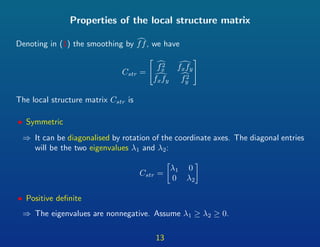
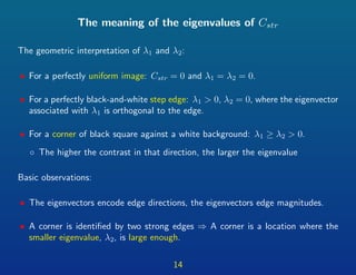
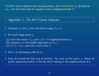
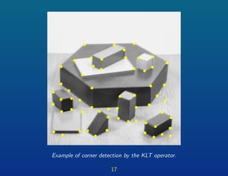
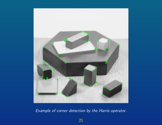
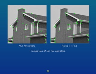
This document provides a summary of corner detection techniques in digital images. It discusses the local structure matrix, which is used in two popular corner detectors: the Kanade-Lucas-Tomasi (KLT) corner detector and the Harris corner detector. Both detectors identify corners as locations where variations of image intensity are high in two orthogonal directions, as measured by the eigenvalues of the local structure matrix. The KLT detector uses an explicit threshold on the smaller eigenvalue, while the Harris detector uses an implicit threshold through a corner response measure. Examples are given to compare the outputs of the two detectors.

1. Institute of Informatics
E¨otv¨os Lor´and University
Budapest, Hungary
Basic Algorithms for Digital Image Analysis:
a course
Dmitrij Csetverikov
with help of Attila Lerch, Judit Verest´oy, Zolt´an Megyesi, Zsolt Jank´o
and Levente Hajder
http://visual.ipan.sztaki.hu

2. Lecture 8: Corner detection
• Zero-crossing edge detector
• Summary of edge detection
• Corner detection in greyscale images
• The local structure matrix
• The KLT corner detector
• The Harris corner detector
• Comparison of the two corner detectors
2

3. Zero-crossing edge detector
2
f(x)
___
Double edge
Zero crossing
Blurred edgeSteep edge
__
dx
df
_
2
d f
dx
-
00
00
+ +
+ +
-
--
Left: Principles of zero-crossing edge detector.
Right: Simple masks for detection of zero-crossings.
3

4. Implementation of the zero crossing filter: Gaussian smoothing followed by
Laplacian filtering.
• Using commutativity and associativity of linear filters and rotation symmetry of
Gaussian filter, we obtain the convolution mask of the zero-crossing operator,
called Laplacian-of-Gaussian (LoG):
wZ(r) = C
r2
σ2
− 1 exp
−r2
2σ2
◦ C: normalisation constant
◦ r2
= x2
+ y2
: square distance from centre of mask
◦ σ is scale parameter: the smaller the σ the finer the edges obtained
• Discrete zero-crossing mask: Threshold wZ(r) at a small level.
⇒ Larger mask obtained for larger σ: For example, when σ = 4 the size of the
mask is about 40 pixels.
4

5. • Another, more efficient but approximate, implementation of the zero-crossing
filter is the difference of two separable Gaussian filters, called DoG.
• Localising the zero-crossings corresponds to edge localisation in gradient-type
edge detectors.
◦ For more precise localisation, one can locally approximate output of LoG filter
by facets (flat patches), then find zero-crossings analytically.
LoG absolute LoG zero DoG zero
Examples of edge detection by 15 × 15 LoG and DoG operators. ‘LoG absolute’ is
absolute value of filter output: dark lines are contours. ‘LoG zero’ was obtained
with removal of weak edges, ‘DoG zero’ without removal.
5

6. Properties of zero crossing edge detector
• The continuous zero-crossing edge detector always gives closed contours.
◦ Reason: Cross-sections of continuous surface at zero level
◦ In principle, this may help in contour following
◦ In practice, many spurious loops appear
• Controlled operator size σ ⇒ Natural edge hierarchy within a scale-space.
◦ Edges may only merge or disappear at rougher scales (larger σ)
◦ This tree-like data structure facilitates structural analysis of image
• Does not provide edge orientation.
◦ Non-maxima suppression and hysteresis threshoding are not applicable
◦ Other ways of post-processing to remove unrealiable edges can be used
6

7. Prewitt 3 × 3 M´er˝o-Vassy 7 × 7 LoG 21 × 21
Canny 3 × 3 Canny 7 × 7 Canny 25 × 25
Examples of edge detection by different operators. The LoG result was obtained
with removal of weak edges. M´er˝o-Vassy is a non-gradient edge detector.
7

8. Summary of edge detection
• 3 × 3 gradient operators (Prewitt, Sobel) are simple and fast. Used when
◦ Fine edges are only needed
◦ Noise level is low
• By varying the σ parameter, the Canny operator can be used
◦ to detect fine as well as rough edges
◦ at different noise levels
• All gradient operators
◦ Provide edge orientation
◦ Need localisation: non-maxima suppression, hysteresis threshoding
• The zero-crossing edge detector
◦ Is supported by neurophysiological experiments
◦ Was popular in the 1980’s
◦ Today, less frequently used in practice
8

9. Corner detection in greyscale images
A reminder:
• Corners are used in shape analysis and motion analysis
◦ Motion is ambiguous at an edge, unambiguous at a corner
◦ Shapes can be approximately reconstructed from their corners
• Two different operations although related operations are called corner detection:
◦ Detection of corners in greyscale images
∗ does not assume extracted contours
◦ Detection of corners in digital curves
∗ assumes extracted contours
This lecture deals with corner detection in greyscale images. Corner detection in
contours will be discussed later.
9

10. Corners, edges, and derivatives of intensity function
Diference between greyscale corners and edges:
• Corners are local image features characterised by locations where variations of
intensity function f(x, y) in both X and Y directions are high.
⇒ Both partial derivatives fx and fy are large
• Edges are locations where the variation of f(x, y) in a certain direction is high,
while the variation in the orthogonal direction is low.
⇒ In an edge oriented along the Y axis, fx is large, while is fy small
Y
X
Y
X
EdgeCorner
A corner and an edge.
10

11. Two selected corner detectors
Different corner detectors exist, but we will only consider two of them:
• The Kanade-Lucas-Tomasi (KLT) operator
• The Harris operator
Reasons:
• Most frequently used: Harris in Europe, KLT in US.
• Can select corners and other interest points.
• Have many application areas, for example:
◦ motion tracking, stereo matching, image database retrieval
• Are relatively simple but still efficient and reliable.
The two operators are closely related and based on the local structure matrix.
11

12. The local structure matrix Cstr
Definition of the local structure matrix (tensor):
Cstr = wG(r; σ) ∗
f2
x fxfy
fxfy f2
y
(1)
Explanation of the definition:
• The derivatives of the intensity function f(x, y) are first calculated in each point.
◦ If necessary, the image is smoothed before taking the derivatives
• Then, the entries of the matrix (f2
x, etc.) are obtained.
• Finally, each of the entries is smoothed (integrated) by Gaussian filter wG(r; σ)
of selected size σ.
◦ Often, a simple box (averaging) filter is used instead of the Gaussian.
12

13. Properties of the local structure matrix
Denoting in (1) the smoothing by ff, we have
Cstr =
f2
x fxfy
fxfy f2
y
The local structure matrix Cstr is
• Symmetric
⇒ It can be diagonalised by rotation of the coordinate axes. The diagonal entries
will be the two eigenvalues λ1 and λ2:
Cstr =
λ1 0
0 λ2
• Positive definite
⇒ The eigenvalues are nonnegative. Assume λ1 ≥ λ2 ≥ 0.
13

14. The meaning of the eigenvalues of Cstr
The geometric interpretation of λ1 and λ2:
• For a perfectly uniform image: Cstr = 0 and λ1 = λ2 = 0.
• For a perfectly black-and-white step edge: λ1 > 0, λ2 = 0, where the eigenvector
associated with λ1 is orthogonal to the edge.
• For a corner of black square against a white background: λ1 ≥ λ2 > 0.
◦ The higher the contrast in that direction, the larger the eigenvalue
Basic observations:
• The eigenvectors encode edge directions, the eigenvectors edge magnitudes.
• A corner is identified by two strong edges ⇒ A corner is a location where the
smaller eigenvalue, λ2, is large enough.
14

15. The KLT corner detector has two parameters: the threshold on λ2, denoted by
λthr, and the linear size of a square window (neighbourhood) D.
Algorithm 1: The KLT Corner Detector
1. Compute fx and fy over the entire image f(x, y).
2. For each image point p:
(a) form the matrix Cstr over a D × D neighbourhood of p;
(b) compute λ2, the smaller eigenvalue of Cstr;
(c) if λ2 > λthr, save the p into a list, L.
3. Sort L in decreasing order of λ2.
4. Scan the sorted list from top to bottom. For each current point, p, delete all
points apperaring further in the list which belong to the neighbourhood of p.
15

16. The output is a list of feature points with the following properties:
• In these points, λ2 > λthr.
• The D-neighbourhoods of these points do not overlap.
Selection of the parameters λthr and D:
• The threshold λthr can be estimated from the histogram of λ2: usually, there is
an obvious valley near zero.
◦ Unfortunately, such valley is not always present
• There is no simple criterion for the window size D. Values between 2 and 10
are adequate in most practical cases.
◦ For large D, the detected corner tends to move away from its actual position
◦ Some corners which are close to each other may be lost
16

17. Example of corner detection by the KLT operator.
17

18. The Harris corner detector
The Harris corner detector (1988) appeared earlier than KLT. KLT is a different
interpretation of the original Harris idea.
Harris defined a measure of corner strength:
H(x, y) = det Cstr − α (trace Cstr)
2
,
where α is a parameter and H ≥ 0 if 0 ≤ α ≤ 0.25.
A corner is detected when
H(x, y) > Hthr,
where Hthr is another parameter, a threshold on corner strength.
Similar to the KLT, the Harris corner detector uses D-neighbourhoods to discard
weak corners in the neighbourhood of a strong corner.
18

19. Parameter of Harris operator and relation to KLT
Assume as before that λ1 ≥ λ2 ≥ 0. Introduce λ1 = λ, λ2 = κλ, 0 ≤ κ ≤ 1.
Using the relations between eigenvalues, determinant and trace of a matrix A
det A =
i
λi
trace A =
i
λi,
we obtain that
H = λ1λ2 − α(λ1 + λ2)2
= λ2
κ − α(1 + κ)2
Assuming that H ≥ 0, we have
0 ≤ α ≤
k
(1 + κ)2
≤ 0.25 and, for small κ, H ≈ λ2
(κ − α) , α κ
19

20. In the Harris operator, α plays a role similar to that of λthr in the KLT operator.
• Larger α ⇒ smaller H ⇒ less sensitive detector: less corners detected.
• Smaller α ⇒ larger H ⇒ more sensitive detector: more corners detected.
Usually, Hthr is set close to zero and fixed, while α is a variable parameter.
original image α = 0.05 α = 0.10
α = 0.20 α = 0.22 α = 0.24
Corner detection by Harris operator: influence of α. (Hthr = 0.)
20

21. Example of corner detection by the Harris operator.
21

22. KLT 40 corners Harris α = 0.2
Comparison of the two operators.
22

23. Summary of corner detection
• The KLT and the Harris corner detectors are conceptually related.
◦ Based on local structure matrix Cstr
◦ Search for points where variations in two orthogonal directions are large
• Difference between the two detectors:
◦ KLT sets explicit threshold on the diagonalised Cstr
◦ Harris sets implicit threshold via corner magnitude H(x, y)
• The KLT detector
◦ usually gives results which are closer to human perception of corners;
◦ is often used for motion tracking in the wide-spread KLT Tracker.
• The Harris detector
◦ provides good repeatability under varying rotation and illumination;
◦ if often used in stereo matching and image database retrieval.
• Both operators may detect interest points other than corners.
23