image segmentation

1. 实验四 图像分割算法基础
1、 实验目的
掌握基本的图象分割方法，观察图象分割的效果；加深对边缘检测、模板匹
配、区域生长的理解；掌握一定的改善分割效果的技巧，如断裂边缘的连接
（Hough 变换）、加入图像特征描述子避免过分割现象（形态学分水岭分割算
法）等；了解医学图像处理相对于其他图像处理的特点。
2、 实验内容
1． 点、线、边沿等灰度不连续性部位的检测；
2． 房屋整体轮廓的检测与描绘；
3． Hough 变换；
3、 知识要点与范例
单色（灰度）图像的分割通常是基于图像强度的两个基本特征：灰阶值的不连续性和
灰度区域的相似性。第一类方法主要是基于图像灰阶值的突然变换（如边缘）来分割图像，
而第二类方法主要是把图像的某个子区域与某预定义的标准进行比较，以二者之间的相似
性指标为指导来划分图像区域：如阈值化技术、面向区域的方法、形态学分水岭分割算法等。
1．点检测
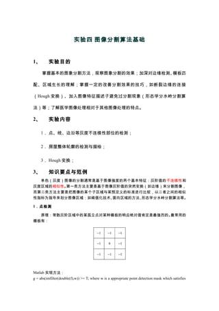
原理：常数灰阶区域中的某孤立点对某种模板的响应绝对值肯定是最强烈的。最常用的
模板有：
Matlab 实现方法：
g = abs(imfilter(double(f),w)) >= T; where w is a appropriate point detection mask which satisfies

2. the above condition.
实例：the detection of isolated bright point in the dark gray area of the northeast quadrant.
(image size: 675*675)
the original image the isolated point detected (only a part displayed)
实例代码：
f=imread('Fig1002(a)(test_pattern_with_single_pixel).tif');
w = [-1 -1 -1; -1 8 -1; -1 -1 -1];
g = abs(imfilter(double(f), w));
T = max(g(:));
g = g>= T;
subplot(121);imshow(f);
title('the original image');
subplot(122);imshow(g(1:end-400, 400:end));
title('the isolated point detected (only a part displayed)');
======================================================================
2．线 (通常假定一个象素厚度) 检测
原理与上同，典型模板有（主要方向性）：
实例：-450
方向线的检测：

3. the original image results from the -45 detecting Zoomed view of the top, left region of (b)
Zoomed view of the bottom, right region of (b) absolute value of (b) -45 line detected
3．边沿检测
方法：使用一阶或者二阶导数。
对一节导数，关键问题是怎样估计水平和垂直方向的梯度 Gx 和 Gy，二阶导数通常使用
Laplacian 算子计算，但是 Laplacian 算子很少单独用来检测边缘，因为其对噪声非常敏感，
而且其结果会产生双边沿，加大了边缘检测的困难。然而，如果 Laplacian 算子能与其他边
缘检测算法相结合，如边缘定位算法，则其是一个强有力的补充。
通常两个标准用来测度图像强度的迅速变化：
(1) 找出强度的一阶导数值大于某个事先阈值标准的位置；
(2) 找出图像二阶导数的跨零点。
IPT 工具箱函数 edge 提供了几种基于上面两种标准的估计器：
其语法为：[g, t] = edge(f, ‘method’, parameters);
这里 ‘method’ 参数包括这几种类型的边缘检测子：Sobel, Prewitt, Roberts, Laplacian of
a Gaussian (LoG), Zero crossings and Canny，前三种的模板见下图：

4. 另一个强有力的边缘检测器：Canny Edge Detector (Canny [1986])，其算法的基本步骤如下：
(1) First, the image is smoothed using a Gaussian filter with a specified standard deviation σ
(2) The local gradient, g(x, y) = [Gx
2
+Gy
2
]1/2
, and edge direction, θ(x, y) = tan-1
(Gy /Gx), are
computed at each point. Any of the first three techniques can be used to computer the Gx and
Gy. An edge point is defined to be a point whose strength is locally maximum in the direction
of the gradient.
(3) The edge points give rise to ridges in the gradient magnitude image. The algorithm then tracks
along the top of these ridges and sets to zero all pixels that are not actually on the ridge top so
as to give a thin line, a process known as nonmaximal suppression. The ridge pixels are the
thresholded using thresholds, T1 and T2, with T1 < T2. Ridge pixels with values greater than
T2 are said to be “strong” edge pixels and pixels between T1 and T2 “weak” edge pixels.
(4) Finally, the algorithm performs edge linking by incorporating the weak pixels that are 8-
connected to strong pixels.
注意：Edge function does not compute edges at ±450
. To compute edges we need to specify
the mask and use imfilter.
4．Hough 变换
In practice, the resulting pixels produced by the methods discussed in the previous sections
seldom characterize an edge completely because of noise, breaks from nonuniform illumination,
and other effects that introduce spurious discontinuities. Hough Transform is one type of linking
procedure to find and link line segments for assembling edge pixels into meaningful edges.
About the principle of Hough transform, please refer to page 586 in textbook.
Instance of Hough transform:
% constructing an image containing 5 isolated foreground pixels in several locaitons:
f = zeros(101, 101);
f(1, 1) = 1, f(101, 1) = 1, f(1, 101) = 1, f(101, 101) = 1, f(51, 51) = 1;
[H, theta, rho] = hough(f); % hough transform
imshow(theta, rho, H, [], 'notruesize');

5. axis on, axis normal;
xlabel('theta'), ylabel('rho');
θ
ρ
-80 -60 -40 -20 0 20 40 60 80
-100
-50
0
50
100
4、 参考程序和参考结果
1．房屋轮廓描绘
代码：
f = imread('Fig1006(a)(building).tif');
[gv, t] = edge(f, 'sobel', 'vertical'); % using threshold computed automatically, here t = 0.0516
subplot(231);imshow(f, []);
title('the original image');
subplot(232);imshow(gv, []);
title('vertical edge with threshold determined automatically');
gv1 = edge(f, 'sobel', 0.15, 'vertical'); % using a specified threshold.
subplot(233);imshow(gv1, []);

6. title('vertical edge with a specified threshold');
gboth = edge(f, 'sobel', 0.15); % edge detection of two directions
subplot(234);imshow(gboth, []);
title('horizontal and vertical edge');
% edge detection of 450
direction using imfilter function
w45 = [-2 -1 0; -1 0 1; 0 1 2];
g45 =imfilter(double(f), w45, 'replicate');
T = 0.3*max(abs(g45(:)));
g45 = g45 >= T;
subplot(235);imshow(g45, []);
title('edge at 45 with imfilter');
wm45 = [ 0 1 2; -1 0 1; -2 -1 0];
g45 =imfilter(double(f), wm45, 'replicate');
T = 0.3*max(abs(g45(:)));
g45 = g45 >= T;
subplot(236);imshow(g45, []);
title('edge at -45 with imfilter');
the original image vertical edge with threshold determined automatically vertical edge with a specified threshold
horizontal and vertical edge edge at 45 with imfilter edge at -45 with imfilter
另一个实验：为比较三种检测方法的相对性能：Sobel, LoG 和 Canny edge detectors，
和为了改善检测效果所需使用的技巧。
% using the default threshold
f = imread('Fig1006(a)(building).tif');
[gs_default, ts] = edge(f, 'sobel'); % ts = 0.074
[gl_default, tl] = edge(f, 'log'); % tl = 0.002 and the default sigma = 0.2
[gc_default, tc] = edge(f, 'canny'); % tc = [0.0189 0.047] and the default sigma = 0.1

7. % using the optimal threshold acquired by manual test
gs_best = edge(f, 'sobel', 0.05);
gl_best = edge(f, 'log', 0.003, 2.25);
gc_best = edge(f, 'canny', [0.04 0.1], 1.5);Sobel operator with deafult threshold
LoG operator with deafult threshold
canny operator with deafult threshold

8. The left column in above figure shows the edge images obtained using the default syntax for the
‘sobel’, ‘log’ and ‘canny’ operator respectively, whereas the right column are the results using
optimal threshold and sigma values obtained by try.
2．Hough 变换用于线检测从而增强边缘的连续性
2.1 Hough transform for peak detection
Peak detection is the first step in using Hough transform for line detection and linking.
However, finding a meaningful set of distinct peaks in a Hough transform can be challenging.
Because of the quantization in space of the digital image and in parameter space of the Hough
transform, as well as the fact that edges in typical images are not perfectly straight, Hough
transform peaks tend to lie in more than one Hough transform cell. One strategy to overcome this
problem is following:
(1) find the HT cell containing the highest value and record its location;
(2) suppress (set to zero) HT cells in the immediate neighborhood of the maximum;
(3) repeat until the desired number of peaks has been found, or until a specified threshold
has been reached.
function [r, c, hnew] = houghpeaks(h, numpeaks, threshold, nhood)
%HOUGHPEAKS Detect peaks in Hough transform.
% [R, C, HNEW] = HOUGHPEAKS(H, NUMPEAKS, THRESHOLD, NHOOD) detects
% peaks in the Hough transform matrix H. NUMPEAKS specifies the
% maximum number of peak locations to look for. Values of H below
% THRESHOLD will not be considered to be peaks. NHOOD is a
% two-element vector specifying the size of the suppression
% neighborhood. This is the neighborhood around each peak that is
% set to zero after the peak is identified. The elements of NHOOD
% must be positive, odd integers. R and C are the row and column
% coordinates of the identified peaks. HNEW is the Hough transform
% with peak neighborhood suppressed.
%
% If NHOOD is omitted, it defaults to the smallest odd values >=
% size(H)/50. If THRESHOLD is omitted, it defaults to
% 0.5*max(H(:)). If NUMPEAKS is omitted, it defaults to 1.
======================================================================
2.2 HT for line detection and linking
For each peak, the first step is to find the location of all nonzero pixels in the image that
contributed to that peak. This purpose can be implemented by the following function:
function [r, c] = houghpixels(f, theta, rho, rbin, cbin)
%HOUGHPIXELS Compute image pixels belonging to Hough transform bin.
% [R, C] = HOUGHPIXELS(F, THETA, RHO, RBIN, CBIN) computes the
% row-column indices (R, C) for nonzero pixels in image F that map
% to a particular Hough transform bin, (RBIN, CBIN). RBIN and CBIN
% are scalars indicating the row-column bin location in the Hough

9. % transform matrix returned by function HOUGH. THETA and RHO are
% the second and third output arguments from the HOUGH function.
[x, y, val] = find(f);
x = x - 1; y = y - 1;
theta_c = theta(cbin) * pi / 180;
rho_xy = x*cos(theta_c) + y*sin(theta_c);
nrho = length(rho);
slope = (nrho - 1)/(rho(end) - rho(1));
rho_bin_index = round(slope*(rho_xy - rho(1)) + 1);
idx = find(rho_bin_index == rbin);
r = x(idx) + 1; c = y(idx) + 1;
The pixels associated with the locations found using houghpixles must be grouped into line
segments, which is programmed into the following function:
function lines = houghlines(f,theta,rho,rr,cc,fillgap,minlength)
%HOUGHLINES Extract line segments based on the Hough transform.
% LINES = HOUGHLINES(F, THETA, RHO, RR, CC, FILLGAP, MINLENGTH)
% extracts line segments in the image F associated with particular
% bins in a Hough transform. THETA and RHO are vectors returned by
% function HOUGH. Vectors RR and CC specify the rows and columns
% of the Hough transform bins to use in searching for line
% segments. If HOUGHLINES finds two line segments associated with
% the same Hough transform bin that are separated by less than
% FILLGAP pixels, HOUGHLINES merges them into a single line
% segment. FILLGAP defaults to 20 if omitted. Merged line
% segments less than MINLENGTH pixels long are discarded.
% MINLENGTH defaults to 40 if omitted.
% LINES is a structure array whose length equals the number of
% merged line segments found. Each element of the structure array
% has these fields:
%
% point1 End-point of the line segment; two-element vector
% point2 End-point of the line segment; two-element vector
% length Distance between point1 and point2
% theta Angle (in degrees) of the Hough transform bin
% rho Rho-axis position of the Hough transform bin
实例：
% first compute and display the Hough transform using a finer spacing than the default.
f = imread('Fig1006(a)(building).tif');

10. gc_best = edge(f, 'canny', [0.04 0.1], 1.5);
[H, theta, rho] = hough(gc_best, 0.5);
imshow(theta, rho, H, [], 'notruesize');
axis on, axis normal;
xlabel('theta'), ylabel('rho')
% next use function houghpeaks to find five HT peaks that are likely to be significant.
[r, c] = houghpeaks(H, 5);
hold on;
plot(theta(c), rho(r), 'linestyle', 'none', 'marker', 's', 'color', 'w');
title('Hough transform with the peak locations superimposed');
% finally, use function houghlines to find and link line segments, and superimpose the line segments on the
original binary image.
lines = houghlines(gc_best, theta, rho, r, c);
figure, imshow(gc_best), hold on;
for k = 1:length(lines)
xy = [lines(k).point1; lines(k).point2];
plot(xy(:, 2), xy(:,1), 'linewidth', 4, 'color', [.6 .6 .6]);
end
title('line segment correspoding to 5 peaks');
Hough transform with the peak locations superimposed
θ
ρ
-80 -60 -40 -20 0 20 40 60 80
-800
-600
-400
-200
0
200
400
600
800

11. line segment correspoding to 5 peaks