Computer Graphics (Hidden surfaces and line removal, Curves and surfaces, Surface Rendering Methods)

CG by Rohit Jasudkar 1
Computer Graphics
21/09/2018
Hidden surfaces and line removal
Curves and surfaces
Surface Rendering methods

Contents
 Hidden surfaces and line removal
• Z buffer Algorithm
• Warnock’s Algorithm
• Painter’s Algorithm
• Backface Removal Algorithm
 Curves and surfaces
• Bezier Curve
• B-splines Curve
 Surface Rendering Methods
• Constant Intensity / Flat Shading
• Gouraurd Shading
• Phong Shading
21/09/2018 CG by Rohit Jasudkar 2

Hidden surfaces and line removal
Overlapping Surfaces
Intersecting Surfaces

Back faced Surfaces
Occluded Surfaces

Hidden Surface Problem
• When we view a picture containing non
transparent objects and surfaces, then we can’t see
those objects from view which are behind from the
objects closer to eye.
• We must remove these hidden surfaces to get
realistic screen image.
• The identification & removal of these surfaces is
called the Hidden-surface problem .
• Techniques used for solving these problems known
as Visible Surface Detection or Hidden Surface
Removal.

Classification of Visible Surface Detection
1. Object space methods
2. Image space methods

Object space methods
• Methods based on comparison of objects for
their 3D positions and dimensions with
respect to a viewing position.
• Efficient for small number of objects but
difficult to implement.
• Depth sorting (Painter Algorithm) , area
subdivision methods (Warnock’s Algorithm).

Image space methods
• Based on the pixels to be drawn on 2D. Try to
determine which object should contribute to that
pixel.
• Running time complexity is the number of pixels
times number of objects.
• Space complexity is two times the number of pixels:
– One array of pixels for the frame buffer
– One array of pixels for the depth buffer
• Depth-buffer (Z-Buffer) and ray casting methods.

Z buffer Algorithm
• Also known as depth -Buffer method.
• Proposed by Mr. Edwin Catmull in 1975
• Z-buffer is like a frame buffer, contain
depths

Basic Z-buffer idea:
• Rasterize every input polygon
• For every pixel in the polygon interior,
calculate its corresponding z value.
• Track depth values of closest polygon
(smallest z) so far
• Update the pixel values with the color of
the polygon whose z value is the closest to
the eye.

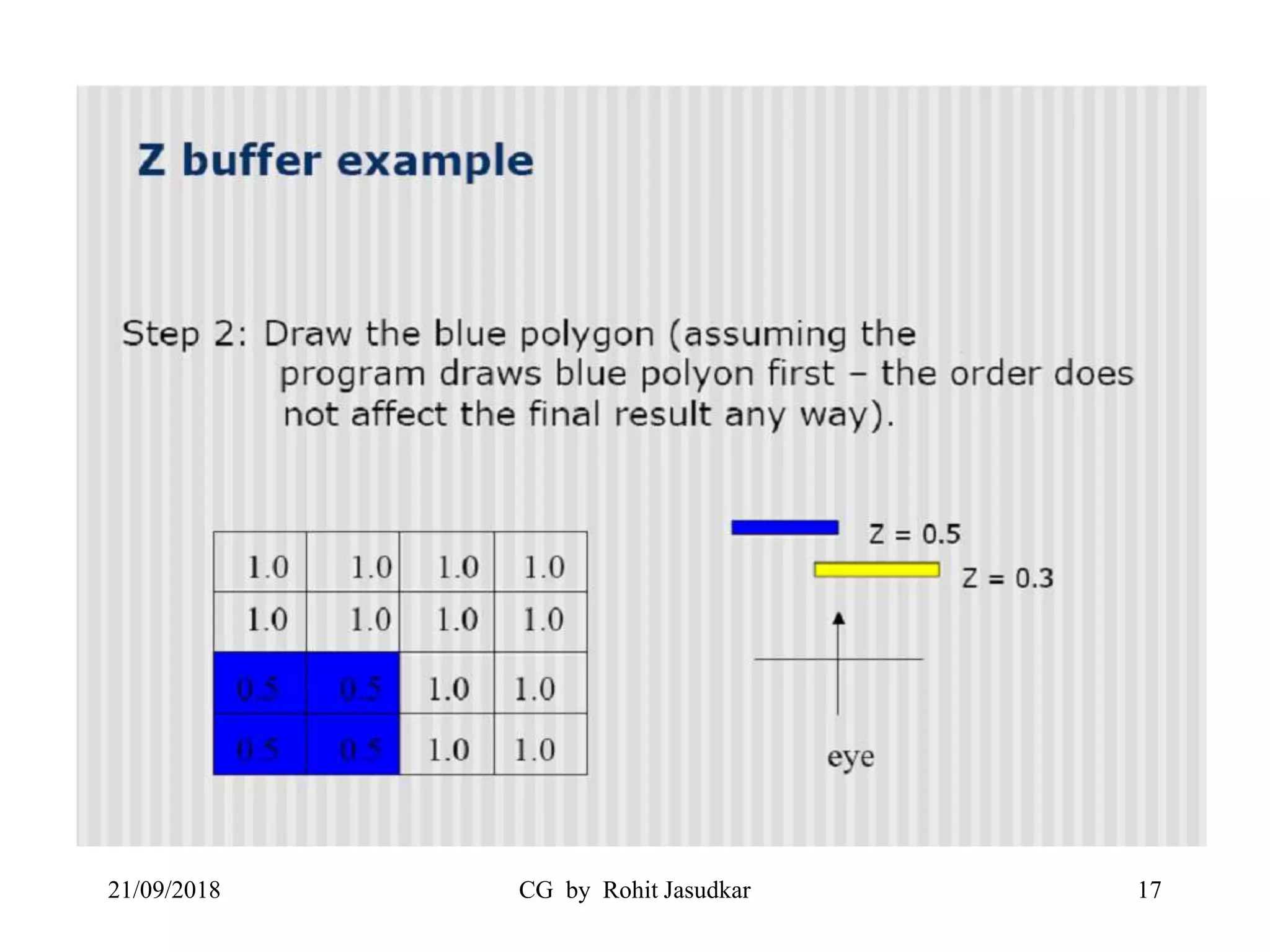
• Two buffers are used
– Frame Buffer (Store Background intensity
or Shades)
– Depth Buffer (Store depth (Z) value of every
visible pixel in image space)
• The z-coordinates (depth values) are
usually normalized to the range [0,1]

Z – Buffer Algorithm
• Initialize the depth buffer and frame buffer so that
for all buffer positions (x ,y ),
depthBuff (x,y) = 1.0, frameBuff (x,y) = bgColor
• Process each polygon in a scene, one at a time
– For each projected (x ,y ) pixel position of a polygon,
calculate the depth z .
– If z < depthBuff (x,y), compute the surface color at that
position and set
– depthBuff (x,y) = z, frameBuff (x,y) = surfCol (x,y)

Calculating depth values (z)
0,
)(
0




C
C
DByAx
z
DCzByAx
Using the polygon surface equation:

Advantages
• No Sorting of polygons required.
• No Object to Object Comparison.
• Can be applied to non polygonal object.
• Simple to use.
• Computing the required depth values is simple.

Disadvantages
• Requires two buffer which makes is
expensive.
• The required z-precision is maintained at
a higher resolution as compared to x,y
precision.
• High memory requirements.

Warnock’s Algorithm
• Developed by John Warnocks.
• Based on the hypothesis of how human eye , brain
combination processes the information present in a
scene.
• Divide-and-conquer strategy: spatial partitioning in
the projection plane
• An area of the projection plane is examined
• If all polygons visible in that area can be easily
decided, they are displayed
• Otherwise, it is recursively decided

At each stage, the projection of each polygon has one of
four relationships to the area of interest (Window)
• Surrounding polygons completely contain the area of
interest
• Intersecting polygons intersect the area of interest
• Contained polygons are completely inside the area
• Disjoint polygons are completely outside the area

For each window
• Disjoint polygons, the window is empty therefore
displayed with background intesity.
• Intersecting polygons can be split into disjoint and
contained polygons.
• If there is only one contained polygon, fill area with
background, then scan-fill polygon area.
• If there is a single surrounding polygon, and no
intersecting or contained polygons, display the
surrounding polygons color.
• There are more than one surrounding polygon in
window, front of all other polygons display the
surrounding polygon color in the area.
• Otherwise subdivide the window.

Painter’s Algorithm
How painter paints objects in the
scene?
• Draw objects from back to
front
• The new object paint will hide
the old object paint.
• It require depth comparisons.

• Also known as Depth sort Algorithm or
Priority Algorithm.
• Two Basic functions:
1. Sort the polygons according to the farthest Z
coordinate
2. Scan convert each polygon in ascending order of
farthest z coordinate (back-to-front)

• Simple algorithm:
– Sort all polygons based on their farthest z coordinate
– Resolve ambiguities (if overlapping of objects occurs)
– Draw the polygons in order from back to front
• This algorithm would be very simple if the z
coordinates of the polygons were guaranteed never
to overlap. Unfortunately that is usually not the
case, which means that step 2 can be somewhat
complex.

Z min

Overlapping Problem

• All polygons whose z extents overlap must be
tested against each other.
• We start with the furthest polygon and call it P.
Polygon P must be compared with every
polygon Q whose z extent overlaps P's z extent.
5 comparisons are made. If any comparison is
true then P can be written before Q.

Test Cases
• 1. Do P and Q's x-extents not overlap?
• 2. Do P and Q's y-extents not overlap?
• 3. Is P entirely on the opposite side of Q's plane from the
viewport?
• 4. Is Q entirely on the same side of P's plane as the viewport?
• 5. Do the projections of P and Q onto the (x,y) plane not
overlap?
If all 5 tests fail we quickly check to see if switching P
and Q will work.

Backface Removal Algorithm
N = Normal Vector of surface plane (N1 and N2)
V = Viewing direction
N1
N 2

if N.V > 0
it is back-face of object from viewing
direction
if N.V < 0
it is front face of object from viewing
direction
Example:
• N1.V < 0 Therefore N1 plane is front face (Visible)
• N2.V > 0 Therefore N2 plane is back face (Invisible)

Curves and surfaces
• A line which is not straight with no sharp
edges is called a curve.
• It is a smoothly flowing line.

Interpolation vs. Approximation
• Interpolation
– Goes through all specified points
– Sounds more logical
– Ex. Lagrange’s, Hermite Interpolation Curve
• Approximation
– Does not go through all points
– Here p1, p2, p3, p4 are control points
– Ex. Bezier , B-spline Approximation Curve

Bezier Curves
• Bezier curve is discovered by the French
engineer Pierre Bézier.
• These curves can be generated under the
control of other points.
• It has global control.
• Approximate tangents by using control points
are used to generate curve.

Cubic Bezier Curve
• The degree of the polynomial defining the curve
segment is one less that the number of defining
polygon point. Therefore, for 4 control points, the
degree of the polynomial is 3, i.e. cubic polynomial.

|
|
|
t = 0.25
t = 0.5
t = 0.75

B-spline Curve
• P0, P1, P2, P3 are the control points.
• X0, X1, X2, X3 are the knot values.
• Q0, Q1, Q2 are the segments of the curve.
To design a B - spline curve, we need a set of control points, a set
of knots and a order of curve(k).

• B-Spline curve uses (n+1) control points
as P0, P1,…….,Pn.
• Order of Curve (k) means, k points
generate a segment.
2 <= k < n+1
• In e.g. k = 2 means that two point P0, P1
generate the segment Q0.
• Degree of polynomial (k - 1)is depends on
order of curve.
• For e.g. if k=3 degree of polynomial=2

• It has local control over the curve.

• Number of segment = n – k + 2
• A B-spline curve is defined as a linear combination of
control points Pi and B-spline basis function Ni, k (t)
given by
• Where,
• {pi: i=0, 1, 2….n} are the control points
• k is the order of the polynomial segments of the B-
spline curve. Order k means that the curve is made up
of piecewise polynomial segments of degree k - 1,
• the Ni,k(t) are the “normalized B-spline blending
functions”. They are described by the order k.

• B- Spline Curve allows us to change the
number of control points without
changing the degree of polynomial.
• As degree of polynomial is depends on
order of curve (k)

Surface Rendering methods
• 3-D image creation phases
– Tessellation.
– Geometry.
– Rendering.
• Shading

What Causes Shading?
• Shading caused by different angles
with light, camera at different points

• The ray is reflected from the object.
• (If the surface is a transparent surface,
the ray is refracted as well as reflected.)

Two types of reflection
• a. Specular/ Regular reflection
• b. Diffused/ Irregular reflection

Illumination model

Constant Intensity / Flat Shading
• Simplest shading algorithm.
• Using an illumination model to determine
the corresponding intensity value for the
incident light.
• Then shade the entire polygon according
to this value.

• Each entire polygon is drawn with the
same colour
• Need to know one normal for the entire
polygon
• It is fast shading method
• Lighting equation used once per polygon

Gouraurd Shading
• Developed in the 1970s by Henri Gouraud.
• It is the interpolation technique.
• Intensity levels are calculated at each vertex
and interpolated across the surface.
• Intensity values for each polygon are matched
with the values of adjacent polygons along the
common edges.
• This eliminates the intensity discontinuities
that can occur in flat shading.

• To render a polygon, Gouraud surface
rendering proceeds as follows:
– Determine the average unit normal vector at each
vertex of the polygon.
– Apply an illumination model at each polygon
vertex to obtain the light intensity at that position.
– Linearly interpolate the vertex intensities over the
projected area of the polygon

• The average unit normal vector at V is
given as:

• Illumination values are linearly
interpolated across each scan-line as
shown in figure

Phong Shading
• A more accurate interpolation based approach for
rendering a polygon was developed by Phong Bui
Tuong.
• Also called as normal-vector interpolation
rendering.
• It interpolates normal vectors instead of intensity
values.
• It requires more calculations and greatly increases
the cost of shading steeply.

• To render a polygon, Phong surface rendering
proceeds as follows:
– Determine the average unit normal vector at each
vertex of the polygon.
– Linearly interpolate the vertex normal over the
projected area of the polygon.
– Apply an illumination model at positions along scan
lines to calculate pixel intensities using the interpolated
normal vectors as shown in figure

Any Questions???

Thank You…

Computer Graphics (Hidden surfaces and line removal, Curves and surfaces, Surface Rendering Methods)

More Related Content

What's hot

Similar to Computer Graphics (Hidden surfaces and line removal, Curves and surfaces, Surface Rendering Methods)

Recently uploaded

Computer Graphics (Hidden surfaces and line removal, Curves and surfaces, Surface Rendering Methods)