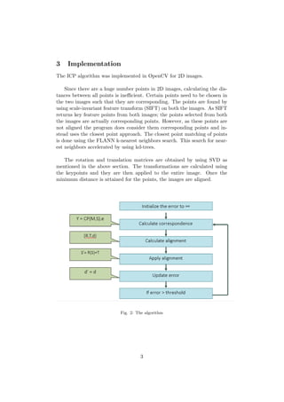
Iterative Closest Point Algorithm
3D Computer Vision - Project Report
Kartik Saxena, Pankaj Gautam
1 Introduction
The objective of this project is to implement the Iterative Closest Point Al-
gorithm (ICP). ICP is used to align partially-overlapping point clouds, given
an initial guess for relative transform. The mesh that is used as reference for
the alignment is called the model and the mesh that is transformed is call the
scene. The algorithm performs the alignment by finding a correspondence
between the model and scene points and calculating the distance between
the those points, and then finding and applying a rotation and translation
to the scene such that the error is minimized. In this project, we present an
implementation of ICP for two-dimensional images.
Fig. 1: A visual representation of ICP
2 The Algorithm
2.1 Finding Corresponding Points
As the two meshes are not aligned, unless specified the correspondence of
points between the two meshes is not known. The algorithm makes an
assumption that there are equal number points both the meshes. There are
different ways of finding the correspondence:
• Closest point: It is assumed that the point in the scene closest to a
point in the model is its correct correspondence.
• Normal Shooting: A normal dropped from the model to the scene
gives the corresponding point.
• Projective: The point in the model intersecting the projection of the
line of joining the camera and the scene point.
The closest point approach is used in this project.
1
2.2 Calculating distances
The algorithm uses simple Euclidean distance for calculating the separation
between the points. Given two corresponding points rm and rs in the model
and scene respectively, the distance is given by:
d(rm, rs) = (xm − xs)2 + (ym − ys)2 + (zm − zs)2
The sum of all distances between corresponding points is to be mini-
mized.
2.3 Finding Rotation and Translation
Once the distances between all the chosen points are calculated, the rota-
tion and translation of the scene is calculated such that the distances are
reduced. There are different ways of finding the rotation and translation
matrices. A technique using singular value decomposition (SVD) is used in
the implementation and is described [5].
Consider M and S as the set of chosen points in the model and scene
respectively. The mean values ¯m and ¯s are calculated. Then the differences
of each point from the mean is obtained
mci = mi − ¯m
sci = si − ¯s
The correlation matrix of of the model and the scene, given by H is
calculated and SVD of the matrix gives the rotation and translation matrices
ˆR and ˆT respectively.
H = McSc
SVD of H gives,
H = UDV
Therefore,
ˆR = V U
ˆT = ¯d − ˆR ¯m
After successive iterations of transforming the scene a minima for the
sum of the distances is reached.
2
3 Implementation
The ICP algorithm was implemented in OpenCV for 2D images.
Since there are a huge number points in 2D images, calculating the dis-
tances between all points is inefficient. Certain points need to be chosen in
the two images such that they are corresponding. The points are found by
using scale-invariant feature transform (SIFT) on both the images. As SIFT
returns key feature points from both images; the points selected from both
the images are actually corresponding points. However, as these points are
not aligned the program does consider them corresponding points and in-
stead uses the closest point approach. The closest point matching of points
is done using the FLANN k-nearest neighbors search. This search for near-
est neighbors accelerated by using kd-trees.
The rotation and translation matrices are obtained by using SVD as
mentioned in the above section. The transformations are calculated using
the keypoints and they are then applied to the entire image. Once the
minimum distance is attained for the points, the images are aligned.
Fig. 2: The algorithm
3
References
[1] ICP, Ronen Gvili, School of Computer Science, Tel Aviv University
[2] FLANN - Fast Library for Approximate Nearest Neighbours
[3] Zhang, Zhengyou (1994). ”Iterative point matching for registration of
free-form curves and surfaces”. International Journal of Computer Vision
(Springer) 13 (12): 119–152.
[4] Rusinkiewicz, S. and Levoy, M. “Efficient Variants of the ICP Algo-
rithm,” pp. 145 - 152 3-D Digital Imaging and Modeling, 2001. Proceedings.
[5] Eggert, D.W., Lorusso, A. and Fisher, R.B. “Estimating 3-D rigid body
transformations: a comparison of four major algorithms,” Machine Vision
and Applications, Volume 9, Issue 5-6, pp. 272-290
[6] “Iterative Closest Point (ICP) for 2D curves with OpenCV,” Shil, R.
[7] “Implementing SIFT in OpenCV,” Utkarsh Sinha, AI Shack
4

Iterative Closest Point Algorithm - analysis and implementation

  • 1.
    Iterative Closest PointAlgorithm 3D Computer Vision - Project Report Kartik Saxena, Pankaj Gautam
  • 2.
    1 Introduction The objectiveof this project is to implement the Iterative Closest Point Al- gorithm (ICP). ICP is used to align partially-overlapping point clouds, given an initial guess for relative transform. The mesh that is used as reference for the alignment is called the model and the mesh that is transformed is call the scene. The algorithm performs the alignment by finding a correspondence between the model and scene points and calculating the distance between the those points, and then finding and applying a rotation and translation to the scene such that the error is minimized. In this project, we present an implementation of ICP for two-dimensional images. Fig. 1: A visual representation of ICP 2 The Algorithm 2.1 Finding Corresponding Points As the two meshes are not aligned, unless specified the correspondence of points between the two meshes is not known. The algorithm makes an assumption that there are equal number points both the meshes. There are different ways of finding the correspondence: • Closest point: It is assumed that the point in the scene closest to a point in the model is its correct correspondence. • Normal Shooting: A normal dropped from the model to the scene gives the corresponding point. • Projective: The point in the model intersecting the projection of the line of joining the camera and the scene point. The closest point approach is used in this project. 1
  • 3.
    2.2 Calculating distances Thealgorithm uses simple Euclidean distance for calculating the separation between the points. Given two corresponding points rm and rs in the model and scene respectively, the distance is given by: d(rm, rs) = (xm − xs)2 + (ym − ys)2 + (zm − zs)2 The sum of all distances between corresponding points is to be mini- mized. 2.3 Finding Rotation and Translation Once the distances between all the chosen points are calculated, the rota- tion and translation of the scene is calculated such that the distances are reduced. There are different ways of finding the rotation and translation matrices. A technique using singular value decomposition (SVD) is used in the implementation and is described [5]. Consider M and S as the set of chosen points in the model and scene respectively. The mean values ¯m and ¯s are calculated. Then the differences of each point from the mean is obtained mci = mi − ¯m sci = si − ¯s The correlation matrix of of the model and the scene, given by H is calculated and SVD of the matrix gives the rotation and translation matrices ˆR and ˆT respectively. H = McSc SVD of H gives, H = UDV Therefore, ˆR = V U ˆT = ¯d − ˆR ¯m After successive iterations of transforming the scene a minima for the sum of the distances is reached. 2
  • 4.
    3 Implementation The ICPalgorithm was implemented in OpenCV for 2D images. Since there are a huge number points in 2D images, calculating the dis- tances between all points is inefficient. Certain points need to be chosen in the two images such that they are corresponding. The points are found by using scale-invariant feature transform (SIFT) on both the images. As SIFT returns key feature points from both images; the points selected from both the images are actually corresponding points. However, as these points are not aligned the program does consider them corresponding points and in- stead uses the closest point approach. The closest point matching of points is done using the FLANN k-nearest neighbors search. This search for near- est neighbors accelerated by using kd-trees. The rotation and translation matrices are obtained by using SVD as mentioned in the above section. The transformations are calculated using the keypoints and they are then applied to the entire image. Once the minimum distance is attained for the points, the images are aligned. Fig. 2: The algorithm 3
  • 5.
    References [1] ICP, RonenGvili, School of Computer Science, Tel Aviv University [2] FLANN - Fast Library for Approximate Nearest Neighbours [3] Zhang, Zhengyou (1994). ”Iterative point matching for registration of free-form curves and surfaces”. International Journal of Computer Vision (Springer) 13 (12): 119–152. [4] Rusinkiewicz, S. and Levoy, M. “Efficient Variants of the ICP Algo- rithm,” pp. 145 - 152 3-D Digital Imaging and Modeling, 2001. Proceedings. [5] Eggert, D.W., Lorusso, A. and Fisher, R.B. “Estimating 3-D rigid body transformations: a comparison of four major algorithms,” Machine Vision and Applications, Volume 9, Issue 5-6, pp. 272-290 [6] “Iterative Closest Point (ICP) for 2D curves with OpenCV,” Shil, R. [7] “Implementing SIFT in OpenCV,” Utkarsh Sinha, AI Shack 4