Masters Thesis

MENG IN ELECTRONIC SYSTEMS, SEPTEMBER 2016 5
Kinect Fusion-Based SLAM
for Mobile Robotics
Matthew Moynihan, Dublin City University
Abstract—The Kinect Fusion algorithm demonstrates the
power of the Kinect device and has since prompted numerous
developments of sophisticated SLAM systems. This investigation
provides a modern example of kinect-based SLAM system design
and provides a comparison between contemporary models as well
as insight into potential future development.
I. INTRODUCTION
THE last five years have seen a drastic change in the state
of the art of Simultaneous Localisation and Mapping
(SLAM) applications in mobile robotics. For two decades
since the early 90’s most SLAM systems featured sparse
point clouds generated by expensive laser range finders and
alignment provided by iterative point matching algorithms and
bayesian filtering techniques. Modern solutions veer greatly
from this approach with the recent increase in demand for
real time, dense 3D mapping algorithms. This demand comes
as a response to the sudden availability of cheap and reliable
devices such as the Microsoft Kinect or Google’s Project
Tango which maximise the potential for RGB pixel data as
well as the potential for depth information.
Modern approaches to SLAM tend to utilise the potential of
combining full color RGB with depth information (RGBD).
One of the most cited contributions to RGBD SLAM tech-
niques is the Kinect Fusion algorithm by Newcombe et al.
[1]. While this approach still uses classic Iterative Closest
Point(ICP)-variants to achieve visual odometry estimation, it
is among the first to provide accurate and dense mapping of
a small 3D volume in real time.
This investigation aims to present a Kinect Fusion-based point
cloud SLAM system capable of mapping larger volumes while
also taking advantage of the Kinect’s ability to track human
targets for use in real world mobile robotics.
II. RELATED WORK
A. Memory Constraints
While Kinect Fusion inspired a wave of new kinect-based
SLAM research, it can be seen as a vital step towards even
more sophisticated design. One immediate limitation of the
Kinect Fusion algorithm is the restricted volume used for re-
construction. This has since been addressed by the Kintinuous
algorithm by Whelan et al. [2] in which the truncated signed
distance function (TSDF) reconstruction volume is redesigned
to incorporate a cyclic memory buffer-style data structure. This
allows the real time reconstruction volume to be translated
along the global model following the camera’s FOV. A differ-
ent approach by Henry et al. [3] compares the application of
Fig. 1. 3D pose graph representation of one of CIPA Labs at DCU.
Sparse Bundle Adjustment (SBA) and the Tree-Base Network
Optimizer (TORO)[4] to the global optimisation of an RGBD
feature-based point cloud map. The latter approach generates
a surfel representation of the global map, a technique which
greatly reduces in post-process rendering.
B. ICP-Variant Point Cloud Alignment
The ICP algorithm as a method for registration of 3D shapes
is most commonly attributed to the 1992 paper by Besl &
McKay [5]. Since its emergence it has largely been considered
the state of the art in point cloud alignment and hence, features
heavily in point cloud based SLAM [6]. In its initial form
the ICP algorithm estimates the transformation between two
sets of 3D points using a point-to-point correspondence. It
has since been improved upon greatly by the introduction of
new constraint models such as the locally planar point-to-plane
model [7] and the Generalised ICP (GICP)[8] plane-to-plane
probabilistic model. Where the original algorithm seeks to
minimise the pointwise euclidean distance between each set,
it is prone to converging on a local minimum solution. Point-
to-plane takes advantage of the locally planar nature of the
real world in order to reduce the likelihood of converging on
local minima. GICP combines the point-to-point and point-to-
plane models into a probabilistic framework which naturally
converges on the most appropriate of the two. This is done by
defining covariance matrices for every point in each dataset
based on the planar properties of both scans.
Kinect Fusion features a multi-scale frame-to-model imple-
mentation of ICP which aligns the current frame to the
reconstruction model by minimising a global point-to-plane
error metric.

III. ICP-VARIANT POINT CLOUD SLAM
The ICP variants presented below extend upon the core
algorithm which is executed as follows.
Primarily the algorithm can be summarised in two key stages:
1) Find corresponding point pairs between each 3D dataset.
2) Find a transformation which minimises the distance cost
function between each corresponding point pair.
These two steps are performed iteratively in order to converge
on a solution which bestbaligns the two point clouds. As
the transformation is applied at each iteration, new point-pair
correspondences must be calculated. Outlier rejection is also
considered in the form of a distance threshold d. Only point-
pairs whose relative distances lie within this threshold are
considered inliers. The use of outlier rejection assumes that
a perfect overlap is not expected as some points in one scan
will naturally not have any correspondence in the other.
The standard point-to-point ICP model from which the follow-
ing variants are derived is presented as Algorithm 1 below.
input : Two 3D Point clouds, reference cloud A = {ai}
and moving cloud B = {bi}
output: The transformation T which aligns B to A
T ← T0;
while Not converged do
for i ← 1 to N do
mi ← FindClosestPointInA(T · bi);
if mi − T · bi ≤ dmax then
wi ← 1;
else
wi ← 0;
end
end
T ← argmin
T i
wi T · bi − mi
2
;
end
Algorithm 1: ICP core algorithm [8]
One major criticism of the standard point-to-point ICP
model is its tendency to converge on a local minimum solution.
This problem when applied to SLAM systems can manifest
itself as a serious cumulative drift. A relatively easy way to
improve this is to implement Algorithm 1 using the improved
point-to-plane model [7] which modifies the cost function as:
T ← argmin
T i
wi ni · (T · bi − mi)
2
where ni is the normal vector (estimated from 6 neighbouring
points) at the correspondence mi. This encourages the algo-
rithm to converge on a more desired local minimum by adding
a planar constraint.
To further reduce the likeliness of converging on a local
minimum, an initial transformation T*
can be fed into the
algorithm input such that it provides an initial estimate for
the final output T. The algorithm as described so far now
forms a baseline for comparison and a platform for the variants
which follow. The general pipeline of this base algorithm,
illustrated in Figure 2. This pipeline indicates that a K-Nearest
Neighbours via Kd-Tree search is performed in order to
find the matching correspondences between the reference and
moving point clouds. While less accurate than an exhaustive
search, it is significantly less computationally expensive and
worth the trade-off for loss of accuracy.
Fig. 2. Core Design Data Flow Diagram. Corresponding Inliers are found via
KNN Kd-Tree search while outliers are removed via dmax treshold condition.
The variants presented below expand on this algorithm by
introducing an initial transformation T∗
by constant velocity
model and by non-linear least squares ICP estimation respec-
tively. The final variant explores the full range of RGBD data
available using the Microsoft Kinect. RGB data in combination
with corresponding depth frame data offers the ability to use
robust feature detectors like SIFT/SURF to extract feature
descriptors with 3D relevance. This can then be expanded
upon to perform 3D ICP alignment enhanced by highly-
corresponding 2D features in a similar manner to the works
of Henry et al. [3].
A. ICP with Constant Velocity Model
The constant velocity model for transformation estimates is
the most intuitive and easiest variant to implement. The model
simply assumes that camera velocity remains constant and
thus the previous transformation is an approximate estimation
of the next. This provides an reasonable estimate of the
translation parameters of the optimum transform. The rotation
parameters are further estimated by approximation of small
angles of rotation between frames and solving the point-to-
plane distance function as before.
B. Non-Linear Least Squares ICP Estimation Model
Both point-to-point and point-to-plane metrics are often
solved by singular value decomposition[9] and linear approx-
imation of small angles respectively. Solving for non-linear
least squares proposes a more accurate solution despite still
converging on a local minimum. While multiple methods exist
for solving non-linear least squares problems, the Levenberg-
Marquradt(LM) approach tends to be the most popular. This
is most likely due to its reasonable computational efficiency
and robustness to harsh initial conditions. The initial estimator
given by this approach is provided by taking advantage of the
LM algorithm’s robustness to initial conditions and solving for
the point-to-point cost function. This is performed iteratively
as in the core ICP algorithm 1 until the solution converges to
within a specific threshold d∗
.

C. RGBD/RANSAC Transform Estimation
Using the full range of data available from the Kinect
device, a combination of 2D feature extraction with 3D
correspondence and RANSAC outlier removal provides
consistently accurate point-pair inliers. This algorithm is
inspired by the FOVIS algorithm developed by Henry et al.
[10]. SURF features are extracted for every source RGB
frame and corresponding target frame. Unique feature matches
are then identified using an exhaustive nearest neighbours
search. Outliers are then excluded using the RANSAC variant
M-estimator SAmple Consensus (MSAC) algorithm [11].
Any image pairs with zero-valued depth correspondence are
also removed.
input : RGBFrameData, depthFrameData
output: T∗
1 srcPoints ←SURFFeatures(srcRGBFrame);
2 trgtPoints ←SURFFeatures(trgtRGBFrame);
3 pairIndxs ←matchFeatures(srcPoints, trgtPoints);
4 inlierIndxs ←estimateMSAC(pairIndxs);
5 srcCloud ←genFeatCloud(inlierIndxs, srcdFrame);
6 trgtCloud ←genFeatCloud(inlierIndxs, srgtdFrame);
7 T∗
←estimateSVDtForm(srcCloud, trgtCloud);
Algorithm 2: RGBD/RANSAC transformation estimator al-
gorithm steps. SURF features are extracted and matched
via K nearest neighbours. Outliers are then removed using
MSAC. Finally, feature clouds are generated from RGB-D
correspondence and aligned using SVD method.
The output of this process is a set of 2D RGB feature
correspondences with associated 3D values which can be
converted into feature-based point clouds. The conversion from
2D depth map to 3D point cloud can be performed using
the Kinect’s intrinsic parameters which are provided in the
Microsoft Kinect v1.8 SDK but can be slightly improved
upon by manual calibration using the following equation.
Where, fx, fy and cx, cy are the focal length and optical center
respectively.
for v ← 1 to range(depthImage.height) do
for u ← 1 to range(depthImage.width) do
Z =depthImage[v, u];
X = (u−cx)·Z
fx
;
Y =
(u−cy)·Z
fy
;
end
end
The rigid transformation which aligns the feature-based
point clouds can then be estimated using the closed-form
least-squares SVD solution by Horn et al. [9]. This rigid
transformation provides the RGBD/RANSAC initial estimator
for the point-to-plane ICP algorithm.
D. Memory Management
MATLAB was the chosen platform for rapid prototype
development. By default, the video input object class in
MATLAB uses a small pre-allocated memory buffer for storing
acquisition data. Two options were explored in order to expand
memory usage. The first option is to quickly offload the
buffer on small frame intervals such as not to interrupt the
next trigger sequence in real time. The second is to write
acquired data directly to disk which was found impractical
going forward with a real time implementation.
For each trigger sequence two large arrays are created,
480x640x3xnframes and 480x640xnframes for colour frames
and depth frames respectively. At the end of each trigger, these
arrays along with the relevant meta data are extracted from the
buffer. The buffer is then cleared for the next sequence while
data from the previous sequences remain in memory. This
technique in combination with an ideal frame rate (dependent
on the average velocity of the camera) allows for large pose-
graph generation.
E. Human Target Tracking and Trajectory Prediction
In order to provide some robustness to dynamic elements in
the reconstruction scene, it was logical to take advantage of
the sophisticated human detection classifiers available within
the Kinect SDK. This feature allows for dynamic segmentation
and 3d tracking of a person walking through the reconstruction
scene. By doing so it enables mask generation such that the
person(s) occluding the scene and otherwise implying non-
rigid frame alignment no longer contribute to the reconstruc-
tion. In addition, tracking data allows for simple trajectory
estimation using Kalman filtering in order to predict possible
pathway interceptions. The algorithm for tracking, masking
and path projection is described as Algorithm 3. The ability
to avoid collision with moving people in an environment is
an essential feature for any SLAM-based autonomous mobile
robotics. The Kinect SDK in combination with MATLAB
allows detection and tracking for up to 6 targets.
input : Kinect Metadata
output: Mask M and trackingCoords
skeletonData ←
extractSekeltonData(kinectMetaData);
if isTracked then
M ← extractSegmentationData(skeletonData) ;
M ← dilate(M);
for i ← 1 to 20 do
trackingCoords ←
extractJointCoordinates(i, skeletonData);
end
end
Algorithm 3: Tracking and masking algorithm. Kinect SDK
provides segmentation of detected human shape into a skele-
ton frame of 20 separate joints.

IV. RESULTS
A series of scrutinous tests were performed in order to
characterise the performance of the system under a variety
of potential real-world applications. In addition to providing
a benchmark for comparing the three aforementioned ICP
estimator variants, additional procedures also examine memory
management and target tracking performance.
A. Hardware Used
All simulations and tests were performed in the MATLAB
environment, on the same platform consisting of a Dell Insp-
iron 15-5548 laptop running 64-bit Windows 10 with an Intel
Core i7-5500U 2.40GHz CPU, 8GB DDR3 RAM and AMD
Radeon R7 M270 4GB DDR3 GPU. The camera used was
a Microsoft Kinect fitted with a custom battery pack DC12V
output for portability.
B. ICP-Variant Performance
For quantitative analysis of rotation, translation and pose
error metrics a popular standard SLAM benchmark dataset
provided by Sturm et al. [12] was used. The ground truth pose
information from this dataset was acquired via an external
motion capture system. All other local datasets described
were captured at 20fps as an acceptable compromise in order
to maximise memory buffer resources without sacrificing
accuracy. The performance of each ICP variant is presented
in tables I and II below. The results obtained show the
frame-wise mean error in translation(m) and rotation(deg)
respectively over 350 frames.
TABLE I
MEAN TRANSLATIONAL ERROR
RGBD(m) ConstV(m) LSQICP(m)
frei1 xyz 0.014601 0.012956 0.013286
frei1 desk 0.019460 0.017139 0.017750
frei2 desk 0.037013 0.010635 0.011306
frei2 large no loop 0.088389 0.025894 0.037033
frei2 360 hemisphere 0.047814 0.036491 0.059924
TABLE II
MEAN ROTATIONAL ERROR
RGBD(deg) ConstV(deg) LSQICP(deg)
frei1 xyz 0.462803 0.412147 0.479754
frei1 desk 0.860328 0.759179 0.840653
frei2 desk 0.389889 0.182279 0.297281
frei2 large no loop 0.527957 0.300519 0.350096
frei2 360 hemisphere 0.308016 0.156127 0.274081
These evaluations were generated using the online version
of the recommended evaluation script[13]. Each frame is
matched to its corresponding ground truth value by timestamp
synchronisation.
C. Memory Management
One simple experiment was conducted to evaluate the opti-
mum number of frames per buffer flush to be used which has
the minimum impact on acquisition. In order to characterise
acquisition performance a single loop of a small area was
performed over 100 frames and repeated for each value of
frames per buffer.
Fig. 3. Processing time between frames for various trigger lengths. Processing
time was recorded after each trigger. Time between trigger sequences is
linearly interpolated.
D. Target Tracking
The base performance of the target tracking and masking
feature was established in ideal conditions i.e. tracking and
masking a single moving target across static frames. Various
tests were then performed to compare the performance under
more stressful conditions such as dynamic movement between
target and camera, multiple targets and occluded targets.
Illustrated in Fig 4 is an experiment to test SLAM performance
during parallel motion with a target.
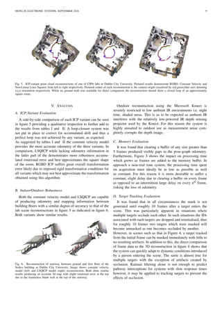
Fig. 4. Tracked target masked out of reconstruction and idicated at frames
2, 50, and 100 in parallel motion from right to left. Camera axes is given by
blue, red, green axes with blue (z-axis) being the optical axis.

Fig. 5. ICP-variant point cloud reconstructions of one of CIPA labs in Dublin City University. Pictured results demonstrate RGBD, Constant Velocity and
Non-Linear Least Squares from left to right respectively. Pictured center of each reconstruction is the camera origin visualised by red,green,blue axes denoting
x,y,z orientation respectively. While no ground truth was available for direct comparison the reconstruction should show a closed loop of an approximately
square room.
V. ANALYSIS
A. ICP-Variant Evaluation
A side-by-side comparison of each ICP variant can be seen
in figure 5 providing a qualitative inspection to further add to
the results from tables I and II. A loop-closure system was
not put in place to correct for accumulated drift and thus a
perfect loop was not achieved by any variant, as expected.
As suggested by tables I and II the constant velocity model
provides the most accurate odometry of the three variants. In
comparison, LSQICP while lacking odometry information in
the latter part of the demonstrates more robustness accumu-
lated rotational error and best approximates the square shape
of the room. RGBD ICP suffers great overall transformation
error likely due to imposed rigid transformation conditions for
all variants which may not best approximate the transformation
obtained using this algorithm.
B. Indoor/Outdoor Robustness
Both the constant velocity model and LSQICP are capable
of producing odometry and mapping information between
building floors with a similar degree of accuracy to that of the
lab scene reconstructions in figure 5 as indicated in figure 6.
Both variants show similar results.
Fig. 6. Reconstruction of stairway between ground and first floor of the
Stokes building at Dublin City University. Image shows constant velocity
model (left) and LSQICP model (right) reconstruction. Both show similar
results producing an accurate 3d map with slight rotational error at the top
due to the featureless blank wall at the top of the stairway.
Outdoor reconstruction using the Microsoft Kinect is
severely restricted to low ambient IR environments i.e. night
time, shaded areas. This is as to be expected as ambient IR
interferes with the relatively low-powered IR depth sensing
projector used by the Kinect. For this reason the system is
highly unsuited to outdoor use as measurement noise com-
pletely corrupts the depth image.
C. Memory Evaluation
It was found that clearing a buffer of any size greater than
5 frames produced visible gaps in the pose-graph odometry.
Furthermore, Figure 3 shows the impact on processing time
which grows as frames are added to the memory buffer. In
approach a near-real time system, the processing time spent
on acquisition must ideally be as low as possible as well
as constant. For this reason it is more desirable to suffer a
constant, slight delay due to clearing a buffer on every frame
as opposed to an intermittent large delay on every nth
frame,
risking the loss of odometry.
D. Target Tracking Evaluation
It was found that in all circumstances the mask is not
generated until roughly 10 frames after a target enters the
scene. This was particularly apparent in situations where
multiple targets occlude each other. In such situations the IDs
associated with each targets are dropped and reinitialised, thus
for roughly 10 frames two targets which were masked will
become unmasked as one becomes occluded by another.
However, in scenes such as that in Figure 4, a target tracked
from the initial frame can be masked immediately with little to
no resulting artifacts. In addition to this, the direct comparison
of frame data to the 3D reconstruction in figure 4 shows that
the system can quickly adapt to dynamic conditions introduced
by a person entering the scene. The same is almost true for
multiple targets with the exception of artifacts created by
occlusion. Kalman filtering alone is not enough to predict
pathway interceptions for systems with slow response times
however, it may be applied to tracking targets to prevent the
effects of occlusion.

VI. CONCLUSIONS
This investigation set out to explore the application of a
gaming-purpose built depth camera to the task of SLAM sys-
tem performance inspired by Kinect Fusion. It sought to draw
comparison between three techniques for ICP initialisation as
well as provide a solution to memory issues and dynamic
reconstruction. Overall, the investigation proposed to suggest
a system design for future use in SLAM for mobile robotics.
In drawing direct comparison with the three ICP variants, the
simplest and most intuitive system using a constant velocity
model emerges with the most accurate results closely followed
by a non-linear least squares estimator method. The current
design featuring RGBD/RANSAC based ICP fails to meet the
minimum standards of the investigation and often results in
unacceptable degrees of error. Two key factors contribute to
this result and must be corrected in future works in order
to produce satisfactory results. The first key factor lies in
the assumption of rigid transformation between frames. While
this is ideally true for static environments, distortions such
as motion blur in acquisition can lead to requiring non-
rigid transformation between frames to achieve the correct
alignment. The second factor lies in the sparseness of the
feature clouds generated by extracting SURF features. While
other feature detectors like Harris or FAST may return a
greater number of keypoints, the consistency of SURF/SIFT
is more desirable. It is instead that the alignment procedure
between sparse clouds must show more robustness than the
current SVD method achieves.
In contrast with the Kinect Fusion algorithm, reconstruction
accuracy is lost in the absence of computationally expensive
rendering. However, it can still be said that the offline CPU-
based prototype presented by this investigation provides a solid
basis for future GPU-based implementation along with the
following suggested additional features and improvements.
A. Future Work
To address the two factors restricting the performance of
RGBD/RANSAC ICP, a more robust, non-rigid alignment
procedure is necessary. Drawing from the work of Henry et al.
in [3], a non-rigid transformation may be estimated by using
a 3D affine transformation fit model for 3D RANSAC outlier
rejection. The best-fit affine transformation returned can then
be used as an estimator for core ICP in future works.
In its current form the system presented performs ICP match-
ing on a frame-by-frame basis. With an appropriately chosen
method for outlier rejction such as RANSAC, it can be ex-
pected that accumulated drift can be reduced using a frame-to-
model based approach such as that used in Kinect Fusion[1].
Further reduction in cumulative drift may be achieved by
implementing the probabilistic constraints proposed by the
GICP algorithm in combination with the establish constant
velocity model.
The approximation of small rotations sacrifices a large degree
of robustness to the roll, pitch, yaw odometry parameters.
While the aforementioned frame-to-model matching improve-
ment may help correct for this, a kalman filter based pose
estimator may be applied as a proposed successor to constant
velocity estimation [14].
For the proposed migration of the system from offline CPU to
online GPU, it will be necessary for failsafe design. It would
require that, if odometry information is lost, the user may
be prompted to return to the last available frame. This has
been accounted for, to some degree, in the current system.
Filters have been put in place which detect unnatural changes
in velocity or error between frame alignment. In such an event
a constant ICP alignment check can be performed between
current frames and the last stored frame. Odometry can be
re-established once an ICP alignment is performed with an
extremely small transformation.
Finally, it may be desirable to apply the system to outdoor
use. As concluded, the microsoft Kinect is unsuitable to this
application. It it therefore proposed to implement more robust
design such as the epipolar IR imaging system presented by
O’Toole et al.[15].
REFERENCES
[1] R. A. Newcombe, S. Izadi, O. Hilliges, D. Molyneaux, D. Kim, A. J.
Davison, P. Kohi, J. Shotton, S. Hodges, and A. Fitzgibbon, “Kinect-
fusion: Real-time dense surface mapping and tracking,” in Mixed and
Augmented Reality (ISMAR), 2011 10th IEEE International Symposium
on, Oct 2011, pp. 127–136.
[2] T. Whelan, M. Kaess, M. Fallon, H. Johannsson, J. Leonard, and
J. McDonald, “Kintinuous: Spatially extended kinectfusion,” 2012.
[3] P. Henry, M. Krainin, E. Herbst, X. Ren, and D. Fox, “Rgb-d mapping:
Using kinect-style depth cameras for dense 3d modeling of indoor
environments,” The International Journal of Robotics Research, vol. 31,
no. 5, pp. 647–663, 2012.
[4] G. Grisetti, S. Grzonka, C. Stachniss, P. Pfaff, and W. Burgard, “Efficient
estimation of accurate maximum likelihood maps in 3d,” in 2007
IEEE/RSJ International Conference on Intelligent Robots and Systems,
Oct 2007, pp. 3472–3478.
[5] P. Besl and N. McKay, “A method for registration of 3d shapes,” vol. 14,
no. 2. IEEE Computer Society, 1992, pp. 239–256.
[6] S. Rusinkiewicz and M. Levoy, “Efficient variants of the icp algorithm,”
in 3-D Digital Imaging and Modeling, 2001. Proceedings. Third Inter-
national Conference on. IEEE, 2001, pp. 145–152.
[7] Y. Chen and G. Medioni, “Object modelling by registration of multiple
range images,” Image and vision computing, vol. 10, no. 3, pp. 145–155,
1992.
[8] A. Segal, D. Haehnel, and S. Thrun, “Generalized-icp.” in Robotics:
Science and Systems, vol. 2, no. 4, 2009.
[9] B. K. Horn, “Closed-form solution of absolute orientation using unit
quaternions,” JOSA A, vol. 4, no. 4, pp. 629–642, 1987.
[10] P. Henry, M. Krainin, E. Herbst, X. Ren, and D. Fox, “Rgb-d mapping:
Using kinect-style depth cameras for dense 3d modeling of indoor
environments,” The International Journal of Robotics Research, vol. 31,
no. 5, pp. 647–663, 2012.
[11] P. H. Torr and A. Zisserman, “Mlesac: A new robust estimator with
application to estimating image geometry,” Computer Vision and Image
Understanding, vol. 78, no. 1, pp. 138–156, 2000.
[12] J. Sturm, N. Engelhard, F. Endres, W. Burgard, and D. Cremers, “A
benchmark for the evaluation of rgb-d slam systems,” in Proc. of the
International Conference on Intelligent Robot Systems (IROS), Oct.
2012.
[13] J. Sturm. (2012) Computer vision group - submission form for
automatic evaluation of rgb-d slam results. [Online]. Available:
http://vision.in.tum.de/data/datasets/rgbd-dataset/online evaluation
[14] Y. Lin, T. Chen, F. Xi, and G. Fu, “Relative pose estimation from points
by kalman filters,” in 2015 IEEE International Conference on Robotics
and Biomimetics (ROBIO), Dec 2015, pp. 1495–1500.
[15] M. O’Toole, S. Achar, S. G. Narasimhan, and K. N. Kutulakos, “Ho-
mogeneous codes for energy-efficient illumination and imaging,” ACM
Transactions on Graphics (TOG), vol. 34, no. 4, p. 35, 2015.

Masters Thesis

More Related Content

What's hot

Viewers also liked

Similar to Masters Thesis

Masters Thesis