control systems template -ppt--pptx Control systems
1.
Course outcome :Calculatethe transfer function of physical systems
CONTROL SYSTEMS
UNIT –I -INTRODUCTION TO CONTROL SYSTEMS
2.
System :
A systemis a combination or an arrangement of different physical components which act
together as a entire unit to achieve certain objective.
• E.g.,
– A classroom is a physical system. A room along with the combination of benches,
blackboard, fans, lighting arrangement etc. can be called as a classroom which acts as
elementary system.
– In a classroom, professor is delivering his lecture, it becomes a control system as; he
tries to regulate, direct or command the students in order to achieve the objective
which is to input good knowledge to the students.
4.
INPUT :It isan applied signal or an excitation signal applied to control system from an external energy
source in order to produce a specified output.
–For each system, there must be excitation and system accepts it as an input
Output :
–It is the particular signal of interest or the actual response
obtained from a control system when input is applied to it.
–for analyzing the behavior of system for such input, it is necessary to define the output of a system.
Plant :
– The portion of a system which is to be controlled or regulated is called as the plant.
– A plant may be a piece of equipment, perhaps just a set of machine parts.
– The purpose of plant is to perform a particular operation.
– E.g., mechanical device, a heating furnace, a chemical reactor, or a spacecraft.
Process:
– Any operation to be controlled is called a process.
– Examples are chemical, economic, and biological processes.
5.
Disturbances :
– Disturbanceis a signal which tends to adversely affect the value of the output of a system.
– Disturbances are undesirable and unavoidable effects beyond our control,
generated from outside process-environment, and from within.
– If such a disturbance is generated within the system itself, it is called as internal disturbance.
– The disturbance generated outside the system acting as an extra input to the system in addition to its normal
input, affecting the output adversely is called as an external disturbance.
– The presence of the disturbance is one of the main reasons of using control.
Controller
:
– The element of the system itself or external to the system which controls the plant or the process is
called as controller.
– E.g., ON/OFF switch to control bulb.
7.
1) Natural ControlSystem
— Universe
— Human Body
2) Manmade Control System
—Vehicles
—Aeroplanes
3)Manual Control Systems
– Room Temperature regulation Via Electric Fan
– Water Level Control
4)Automatic Control System
– Room Temperature regulation Via A.C
– Washing Machines
5) Open-Loop Control System
– Washing Machine
– Toaster
– Electric Fan
6) Closed-loop Control System
– Refrigerator
– Auto-pilot system
8.
7.Linear Vs NonlinearControl System
A Control System in which output varies linearly with the input is called a linear control system.
8)Time variant and Time invariant systems
When the characteristics of the system do not depend upon time itself then the system is said
to time invariant control system.
Time varying control system is a system in which one or more parameters vary with time.
9.
• Any physicalsystem which does not automatically correct for variation in its output, is
called an open-loop system.
• Such a system may be represented by the block diagram as shown in Fig.
• In these systems, output is dependent on input but controlling action or input is totally independent of the
output or changes in output of the system.
• In these systems the output remains constant for a constant input signal provided the external conditions
remain unaltered.
• In any open-loop control system the output is not compared with the reference input. As a result, the accuracy
of the system depends on calibration.
10.
• In thepresence of disturbances, an open-loop control system will not perform the desired task. Open-loop
control can be used, in practice, only if the relationship between the input and output is known and if there
are neither internal nor external disturbances.
• Clearly, such systems are not feedback control systems. Note that anycontrol system that operates on a time
basis is open loop.
• For instance, traffic control by means of signals operated on a time basis is an example of open-loop
control.
Advantages:
The advantages of open loop control system are,
1) Such systems are simple in construction.
2) Very much convenient when output is difficult to measure.
3) Such systems are easy from maintenance point of view.
4) Generally these are not troubled with the problems of stability.
5) Such systems are simple to design and hence economical.
11.
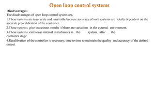
Disadvantages:
The disadvantages ofopen loop control system are,
1.These systems are inaccurate and unreliable because accuracy of such systems are totally dependent on the
accurate pre-calibration of the controller.
2.These systems give inaccurate results if there are variations in the external environment.
3.These systems cant sense internal disturbances in the system, after the
controller stage.
4.Recalibration of the controller is necessary, time to time to maintain the quality and accuracy of the desired
output.
12.
AUTOMATIC TOSTER
•In thissystem, the quality of toast depends upon the time for which the toast is heated.
•Depending on the time setting, bread is simply heated in this system.
•The toast quality is to be judged by the user and has no effect on the inputs.
13.
Traffic Light Controller
•Atraffic flow control system used on roads is time dependent.
•The traffic on the road becomes mobile or stationary depending on the duration and sequence of lamp glow.
•The sequence and duration are controlled by relays which are
predetermined and
•not dependent on the rush on the road.
14.
Feedback Control Systems.
•Asystem that maintains a prescribed relationship between the output and the reference input by comparing
them and using the difference as a means of control is
called a feedback control system.
Closed-Loop Control Systems.
•Feedback control systems are often referred to as closed-loop control systems.
•In practice, the terms feedback control and closed-loop control are used interchangeably.
•In a closed-loop control system the actuating error signal (which is the difference between the input signal and
the feedback signal) is fed to the controller so as to reduce the error and bring the output of the system to a
desired value.
•The term closed-loop control always implies the use of feedback control action in order to reduce system error.
15.
The various signalsare,
r(t) = Reference input
e(t) = Error signal
c(t) = Controlled output
m(t) = Manipulated signal
b(t) = Feedback signal
16.
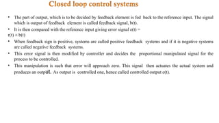
• The partof output, which is to be decided by feedback element is fed back to the reference input. The signal
which is output of feedback element is called feedback signal, b(t).
• It is then compared with the reference input giving error signal e(t) =
r(t) ± b(t)
• When feedback sign is positive, systems are called positive feedback systems and if it is negative systems
are called negative feedback systems.
• This error signal is then modified by controller and decides the proportional manipulated signal for the
process to be controlled.
• This manipulation is such that error will approach zero. This signal then actuates the actual system and
produces an output. As output is controlled one, hence called controlled output c(t).
17.
Advantages
1.Accuracy of thesesystems is always very high because controller modifies and manipulates the actuating
signal such that error in the system will be zero.
2.closed loop system senses environmental changes, as well as internal disturbances and accordingly modifies
the error.
3.There is reduced effect of nonlinearities and distortions.
4.Bandwidth (operating frequency zone) for such system is very high.
Disadvantages
5.systems are complicated and time consuming from design point of view and hence costlier.
6.Due to feedback, system tries to correct the error from time to time. Tendency to overcorrect the error may
cause oscillations without bound in the system.
7.System has to be designed taking into consideration problems of instability due tofeedback.
8.The stability problems are severe and must be taken care of while designing the system.
18.
Human Being
•The bestexample is human being. If a person wants to reach for a book on the table, Position of the book is
given as the reference.
•Feedback signal from eyes, compares the actual position of hands with reference position. Error signal is
given to brain.
•Brain manipulates this error and gives signal to the hands. This process continues till the position of the hands
get achieved appropriately.
19.
Home Heating System
•Inthis system, the heating system is operated by a valve.
•The actual temperature is sensed by a thermal sensor and compared with the desired temperature.
•The difference between the two, actuates the valve mechanism to change the temperature as per
the requirement.
20.
Open Loop ClosedLoop
Any change in output has no effect
on the input i.e. feedback does not exists.
Changes in output, affects the input
which is possible by use of feedback.
Output measurement is not
required for operation of system.
Output measurement is necessary.
Feedback element is absent. Feedback element is present.
Error detector is absent. Error detector is necessary.
It is inaccurate and unreliable. Highly accurate and reliable.
Highly sensitive to the disturbances. Less sensitive to the disturbances.
Bandwidth is small. Bandwidth is large.
Simple to construct and cheap. Complicated to design and hence costly.
Generally are stable in nature. Stability is the major
consideration while designing
Highly affected by nonlinearities. Reduced effect of nonlinearities.
21.
Course outcome :Calculatethe transfer function of physical systems
CONTROL SYSTEMS
UNIT –I
Topic name : Transfer Function of Physical Systems
Connected Co : R16C212.1
Connected POS :PO1,PO2
MRS.V.BINDU
Asst.Professor
EEE
23.
Objectives
•To learn abouttransfer functions.
•To develop mathematical models from schematics of physical system.
Overview
•Review on Laplace transform
•Electric network
•Translational mechanical system
•Rotational mechanical system
•You will learn how to develop mathematical model.
•Present mathematical representation where the input, output and system are different and separate.
•Solving problems in group and individual
Electric network
Translational mechanical system
Rotational mechanical system
24.
Electric Network TransferFunctions
• We are only going to apply transfer function to the mathematical modelling of electric circuits for passive
networks (resistor, capacitor and inductor).
• We will look at a circuit and decide the input and the output.We will use Kirchhoff’s laws as our guiding
principles
Component Voltage
-
Current
Current-
voltage
Current-
voltage
Impedance
Z(s)=
V(s)/I(s)
Admittance
Y(s)=
I(s)/V(s)
Transfer Function : It is defined as the ratio of Input to output expressed in s domain by neglecting initial
conditions
25.
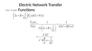
Electric Network Transfer
Functions
Findthe transfer function relating the capacitor voltage, Vc(s), to the input voltage, V(s), in figure below
Redraw the circuit using Laplace transform. Replace the component values with their impedance values.
26.
Determine the inputand the output for the circuit. For this circuit, Input is V(s) Output is
VC(s)
Next, we write a mesh equation using the impedance as we would use resistor values in a
purely resistive circuit.
Electric Network Transfer
Functions
Vc (s) = I (s)
1
Cs
⎜ Ls + R
+
1
⎞
Cs ⎠
⎟I (s) = V
(s)
27.
I (s) =VC (s)Cs
Electric Network Transfer
Functions
28.
We can alsopresent our answer in block
diagram
Electric Network Transfer
Functions
TRANSLATIONAL MECHANICAL SYSTEMTRANSFER FUNCTION
We are going to model translational mechanical system by a transfer function.
In electrical we have three passive elements, resistor, capacitor and inductor. In mechanical we have
spring, mass and viscous damper.
35.
We aregoing to find the transfer function for a mechanical system in term of force-displacement
(i.e. forces are written in terms of displacement)
TRANSLATIONAL MECHANICAL SYSTEM TRANSFER FUNCTION
Mass
f(t) represents the applied force, x(t) represents the displacement, and M represents the mass.
Then, in accordance with Newton’s second law,
Where v(t) is velocity and a(t) is acceleration. It is assumed that the mass is rigid at the top connection
point and that cannot move relative to the bottom connection point.
36.
• Damper isthe damping elements and damping is the friction existing in
physical systems whenever mechanical system moves on sliding surface. The
friction encountered is of many types, namely stiction, coulomb friction and
viscous friction force
• In friction elements, the top connection point can move relative to the bottom
connection point. Hence two displacement variables are required to describe
the motion of these elements, where B is the damping coefficient
TRANSLATIONAL MECHANICAL SYSTEM TRANSFER FUNCTION
Spring
The final translational mechanical element is a spring. The ideal spring gives the
elastic deformation of a body. The defining equation from Hooke’s law, is given
by
37.
Force-velocity, force- displacement,and impedance translational relationships for springs, viscous dampers,
and mass
TRANSLATIONAL MECHANICAL SYSTEM TRANSFER FUNCTION
Steps involved insolving the problem
TRANSLATIONAL MECHANICAL SYSTEM TRANSFER FUNCTION
Draw a free body diagram, placing on the body all forces that act on the body either in the direction of
motion or opposite to it.
Use Newton’s law to form a differential equation of motion by summing the forces and setting the sum
equal to zero.
Assume zero initial conditions, we change the differential equation into Laplace form.
The equation in Laplace form is
(Ms2
+ fvs + K ) X (s) = F (s)
40.
Solving for thetransfer function
TRANSLATIONAL MECHANICAL SYSTEM TRANSFER FUNCTION
a. Forces onM2due only to motion of M2;
b. forces on M2 due only to motion of M1 (sharing);
c. all forces on M2
TRANSLATIONAL MECHANICAL SYSTEM TRANSFER FUNCTION
ROTATIONAL MECHANICAL SYSTEMTRANSFER FUNCTION
We are going to solve for rotational mechanical system using the same way as the translational mechanical
systems except
•
In translational mechanical system we have three elements; spring, damper and mass. In rotational
mechanical system also we have; spring, damper and inertia.
Torque replaces force
Angular displacement replaces translational displacement
45.
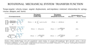
ROTATIONAL MECHANICAL SYSTEMTRANSFER FUNCTION
Torque-angular velocity, torque- angular displacement, and impedance rotational relationships for springs,
viscous dampers, and inertia
46.
ROTATIONAL MECHANICAL SYSTEMTRANSFER FUNCTION
Assumption
Anti-clockwise movement is assumed to be positive
EXAMPLE Find the transfer function, θ(s)/T(s)
ROTATIONAL MECHANICAL SYSTEMTRANSFER FUNCTION
a.Torques on J1 due only to the
motion of J1
b.torques on J1 due only to the
motion of J2
c.final free-body diagram for J1
• Signal-flow graphsare an alternative to block diagrams.
• Signal flow graphs are a pictorial representation of the simultaneous equations describing a
system.
• Signal flow graphs display the transmission of signals through the system, as does the block
diagrams, but it is easier to draw and easier to manipulate than the block diagrams.
• Unlike block diagrams, which consist of blocks, signals, summing junctions, and pickoff
points, a signal-flow graph consists only of branches, which represent systems, and nodes,
which represent signals.
Introduction
55.
Fundamentals of SignalFlow Graphs
• Consider a simple equation below and draw its signal flow graph:
Xi = AijXj
• The signal flow graph of the equation is shown below;
• Every variable in a signal flow graph is designed by a Node.
• Every transmission function in a signal flow graph is designed by a Branch.
• Branches are always unidirectional.
• The arrow in the branch denotes the direction of the signal flow.
• The variables Xi and Xj are represented by a small dot or circle called a Node.
• The transmission function Aij is represented by a line with an arrow called a Branch.
• The Node Xi is called input node and Node Xj is called output node.
56.
Signal Flow GraphAlgebra
1. The Addition Rule:
•The value of the variable designated by a node is equal to the sum of all signals entering the node. This can be
represented as;
•Example: The signal flow graph for the equation of a line in rectangular coordinates, Y = mX + b, is given below.
Since b is a constant it may be represent a node or a transmission function.
57.
2. The TransmissionRule:
•The value of the variable designed by a node is transmitted on every branch leaving that node.
•Example: The signal flow graph of the simultaneous equations, Y = 3X, and, Z = -4X, is given
in the figure below.
Signal Flow Graph Algebra
58.
3. The MultiplicationRule:
•A cascaded or series connection of n-1 branches with transmission functions ,
,can be replace by a single branch with a new transmission function equal to the product of
the old ones. That is
•Example: The signal flow graph of the simultaneous equations Y = 10X, Z = -20Y, is given in
Signal Flow Graph Algebra
59.
Terminologies
• An inputnode or source contain only the outgoing branches. i.e., X1
• An output node or sink contain only the incoming branches. i.e., X4
• A path is a continuous, unidirectional succession of branches along which no node is passed more than ones. i.e.,
X1 to X2 to X3 to X4, X2 to X3 back to X2, X1 to X2 to X4, are paths.
• A forward path is a path from the input node to the output node. i.e.,
X1 to X2 to X3 to X4, and X1 to X2 to X4, are forward paths.
60.
• A feedbackpath or feedback loop is a path which originates and terminates on the same node. i.e.; X2
to X3 and back to X2 is a feedback path.
• A self-loop is a feedback loop consisting of a single branch. i.e.; A33 is a self loop.
• The gain of a branch is the transmission function of that branch when the transmission function is a
multiplicative operator. i.e., A33
• The path gain is the product of branch gains encountered in traversing a path. i.e.,
X1 to X2 to X3 to X4 is A21A32A43
• The loop gain is the product of the branch gains of the loop. i.e., the loop gain of the feedback loop from
X2 to X3 and back to X2 is A32A23.
Terminologies
61.
Converting Cascaded BlockDiagram into a Signal Flow Graph:
• First thing is to draw the signal nodes for the system.
• Next thing is to interconnect the signal nodes with system branches.
• The signal nodes for the system are shown in figure (a).
• The interconnection of the nodes with branches that represent the subsystem is shown in figure (b).
62.
Converting Parallel SystemBlock Diagram into a Signal Flow Graph
• First thing is to draw the signal nodes for the system.
• Next thing is to interconnect the signal nodes with system branches.
• The signal nodes for the system are shown in figure (c).
• The interconnection of the nodes with branches that represent the subsystem is shown in figure (d).
63.
Converting Feedback SystemBlock Diagram into a Signal Flow Graph:
• First thing is to draw the signal nodes for the system.
• Next thing is to interconnect the signal nodes with system branches.
• The signal nodes for the system are shown in figure (e).
• The interconnection of the nodes with branches that represent the subsystem is shown in figure (f).
• If desired,simplify the signal-flow graph to the one shown in Figure (c) by eliminating signals that have a
single flow in and a single flow out, such as V2(s), V6(s), V7(s), and V8(s).
66.
Mason’s Rule (Mason,1953)
• The transfer function, T = C(s)/R(s), of a system represented by a signal-flow graph is;
i = number of forward paths.
Pi = the i th forward-path gain.
Pjk = j th possible product of k no ntouching loop gains.
∆ = 1 - ∑Pj1 + ∑Pj2 - ∑Pj3 +…..
= 1 - ∑ loop gains + ∑ gain products of two non touching loops - ∑ gain products of three non touching
loops + . . .
∆i = ∆ - ∑ loop gain terms in ∆ that touch the i th forward path: In other words;
∆i is formed by eliminating from ∆ those loop gains that touch the i th forward path.
• Two loops, paths, or loop and a path are said to be non touching if they have no nodes in common.
• ∆ is called the signal flow graph determinant or characteristic function. Since ∆=0 is the system characteristic
equation.
67.
Example-3: Consider thesignal flow graph below and identify the
following;
• There are four loop gains;
• There are two forward path gains;
• Nontouching loop gains;
69.
Example-4: Construct thesignal flow graph of the block diagram of the canonical feedback control system
and find the control ratio C/R.
70.
Example-5: Determine thecontrol ratio C/R and the canonical block diagram
of the feedback control system.
Course outcome :Design of state space models
CONTROL SYSTEMS
UNIT –VI- STATE SPACE EQUATONS
Connected Co : R16C212.16
Connected POS :PO1,PO2,P03
MRS.V.BINDU
Asst.Professor
EEE
76.
THE GENERAL STATE-SPACEREPRESENTATION
System variable
Any variable that responds to an input or initial conditions in a system
State Variables
The smallest set of linearly independent system variables Such that the values of the members
of the set at time to along with known forcing functions completely determine the value of all
system variables for all t≥to
State Space
The n-dimension space whose axes are the state variables.(e.g. vR and vC)
State Equation
A set of n simultaneous, first order differential equations with n variables, where n variables to
be solved are the state variables.
Output Equation
The algebraic equations that expresses the output variables of a system as linear combinations of the state
variables and the inputs.
77.
THE GENERAL STATE-SPACEREPRESENTATION
=Ax + Bu
ẋ --- STATE EQUATION
y=Cx + Du ---OUTPUT EQUATION
for t≥to and initial conditions x(to),
where x=state vector
=derivative of the state vector with respect to time
ẋ
y=output vector
u=input or control vector A=system matrix
B=input matrix
C=output matrix
D= feedforward matrix
78.
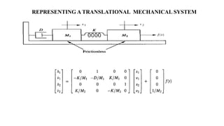
REPRESENTING AN ELECTRICALNETWORK
Problem
Given the electrical network, find a state-space representation if the output is the current
through the resistor.
v(t)
C
79.
Step 1
Label allthe branches currents in the network.
REPRESENTING AN ELECTRICAL NETWORK
iL(t
)
iL(t)
iR(t)
iC(t)
L
R
80.
Step 2
Select thestate variables by writing the derivative equation for all energy storage elements,
that is, the inductor and the capacitor.
REPRESENTING AN ELECTRICAL NETWORK
Step 3
Apply network theory, such as Kirchhoffs voltage and current laws
81.
Step 4
Substitute theresults to obtain the following state equations
REPRESENTING AN ELECTRICAL NETWORK
82.
Step 5
Find theoutput equation.
REPRESENTING AN ELECTRICAL NETWORK
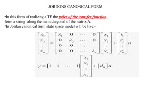
JORDONS CANONICAL FORM
•Inthis form of realizing a TF the poles of the transfer function
form a string along the main diagonal of the matrix A.
•In Jordan canonical form state space model will be like:-
Course outcome :Determination of stability by polar plot
CONTROL SYSTEMS
UNIT –VI- FREQUENCY RESPONSE ANALYSIS
Connected Co : R16C212.16
Connected POS :PO1,PO2,P03
MRS.V.BINDU
Asst.Professor
EEE
• The polarplot of sinusoidal transfer function G(jω) is a plot of the magnitude of G(jω) verses
the phase angle of G(jω) on polar coordinates as ω is varied from zero to infinity.
• Therefore it is the locus of as ω is varied from zero to infinity.
• As
• So it is the plot of vector as ω is varied from zero to infinity
INTRODUCTION
100.
STEPS TO DRAWPOLAR PLOT
• Step 1: Determine the T.F G(s)
• Step 2: Put s=jω in the G(s)
• Step 3: At ω=0 & ω=∞ find by &
• Step 4: Rationalize the function G(jω) and separate the real and imaginary parts
• Step 5: Put Re [G(jω) ]=0, determine the frequency at which plot intersects the Im axis and calculate
intersection value by putting the above calculated frequency in G(jω)
• Step 7: Put Im [G(jω) ]=0, determine the frequency at which plot intersects the real axis and
calculate intersection value by putting the above calculated frequency in G(jω)
• Step 8: Sketch the Polar Plot with the help of above information
101.
Polar Plot forType 0 System
• Let
• Step 1: Put s=jω
• Step 2: Taking the limit for magnitude of G(jω)
102.
Type 0 system
•Step 3: Taking the limit of the Phase Angle of G(jω)
103.
Type 0 system
•Step 4: Separate the real and Im part of G(jω)
• Step 5: Put Re [G(jω)]=0
• Step 2:Taking the limit for magnitude of G(jω)
• Step 3: Taking the limit of the Phase Angle of G(jω)
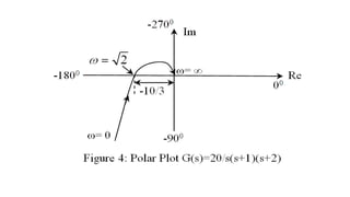
Sketch the polar plot for G(s)=20/s(s+1)(s+2)
Solution:
Step 1: Put s=jω
EXAMPLES
112.
• Step 4:Separate the real and Im part
of G(jω)
By: P.T.KRISHNA SAI, EEE, DIET.
Step 5: Put Im [G(jω)]=0
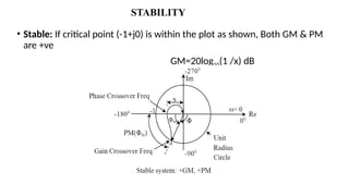
• Phase CrossoverFrequency (ωp) : The frequency where a polar plot
intersects the –ve real axis is called phase crossover frequency
• Gain Crossover Frequency (ωg) : The frequency where a polar plot
intersects the unit circle is called gain crossover frequency
So at ωg
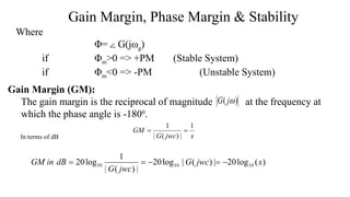
Gain Margin, Phase Margin & Stability
Phase Margin (PM):
Phase margin is that amount of additional phase lag at the gain crossover
frequency required to bring the system to the verge of instability (marginally
stabile)
Φm=1800
+Φ
116.
Where
Φ= G(jω
∠ g)
ifΦm>0 => +PM (Stable System)
if Φm<0 => -PM (Unstable System)
Gain Margin, Phase Margin & Stability
Gain Margin (GM):
The gain margin is the reciprocal of magnitude at the frequency at
which the phase angle is -1800
.
In terms of dB
117.
STABILITY
• Stable: Ifcritical point (-1+j0) is within the plot as shown, Both GM & PM
are +ve
GM=20log10(1 /x) dB
118.
Unstable: If criticalpoint (-1+j0) is outside the plot as shown,
Both GM & PM are -ve
GM=20log10(1 /x) dB
STABILITY
COURSE OUTCOME :DETERMINATION OF STABILITY BY ROUTH CRITERIA
CONTROL SYSTEMS
UNIT –III - TIME DOMAIN ANALYSIS
Connected Co : R16C212.3
Connected POS :PO1,PO2,P03
MRS.V.BINDU
Asst.Professor
EEE
Objective
To determine thestability of a system represented as a transfer function.
A system is stable if every bounded input yields a bounded output. We call this statement
the bounded-input, bounded-output (BIBO).
Using the total response (BIBO)
A system is stable if every bounded input yields a bounded output.
A system is unstable if any bounded input yields an unbounded output.
STABILITY
123.
We can alsodetermine the stability of a system based on the system poles.
Stable systems have closed-loop transfer functions with poles only in the left half-
plane.
Unstable systems have closed-loop transfer functions with at least one pole in the right
half-plane and/or poles of multiplicity greater than 1 on the imaginary axis.
Marginally stable systems have closed-loop transfer functions with only imaginary
axis poles of multiplicity 1 and poles in the left half- plane.
STABILITY
A method tofind the stability without solving for the roots of the system is
called Routh-Hurwitz Criterion.
We can use Routh-Hurwitz criterion method to find how many closed-loop
system poles are in the LHP, RHP and on the jω-axis
Disadvantage : We cannot find their coordinates
The method requires two steps:
Generate a data table called a Routh table
Interpret the Routh table to tell how many close-loop system poles are in
the left half- plane, the right half-plane, and on the jω-axis
ROUTH-HURWITZ CRITERION
128.
Example
displays an equivalentclosed loop transfer function.
In order to use Routh table we are only going to focus on the denominator.
Equivalent closed-loop transfer function
ROUTH-HURWITZ CRITERION
129.
First step (1)
Basedon the denominator in Figure the highest power for s is 4, so we can
draw initial table based on this information. We label the row starting with
the highest power to s0
.
s4
s3
s2
s1
s0
ROUTH-HURWITZ CRITERION
130.
Input the coefficientvalues for each s horizontally starting with the coefficient
of the highest power of s in the first row, alternating the coefficients.
s4
s3
s2
s1
s0
a4
a3
a2
a1
a0
0
ROUTH-HURWITZ CRITERION
131.
Remaining entries arefilled as follows. Each entry is a negative
determinant of entries in the previous two rows divided by the entry in the
first column directly above the calculated row.
ROUTH-HURWITZ CRITERION
Interpreting the basicRouth table
In this case, the Routh table applies to the systems with poles in the left and right
half- planes.
Routh-Hurwitz criterion declares that the number of roots of the polynomial that
are in the right half-plane is equal to the number of sign changes in the first
column.
ROUTH-HURWITZ CRITERION
142.
Example 6.1
Make aRouth table for the system below
Answer:
get the closed-loop transfer function
ROUTH-HURWITZ CRITERION
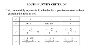
143.
We can multiplyany row in Routh table by a positive constant without
changing the rows below.
ROUTH-HURWITZ CRITERION
144.
If theclosed-loop transfer function has all poles in the left half of the s-
plane, the system is stable.
The system is stable if there are no sign changes in the first column of the
Routh table. Example:
ROUTH-HURWITZ CRITERION
145.
+
-
-
+
Based on thetable, there are two sign changes in the first column. So there are
two poles exist in the right half plane.Which means the system is unstable.
ROUTH-HURWITZ CRITERION
146.
Two special casescan occur:
Routh table has zero only in the first column of
a row
• s3
• s2
s1
Routh table has an entire row that consists of
zeros.
1 3 0
3 4 0
0 1 2
s3
s2
0
1 3
3 4
0
0
0
0
ROUTH-HURWITZ CRITERION: SPECIAL
CASES
147.
Zero only inthe first column
There are two methods that can be used to solve a Routh table that
has zero only in the first column.
1. Stability via epsilon method
2. Stability via reverse coefficients
ROUTH-HURWITZ CRITERION: SPECIAL
CASES
148.
Zero only inthe first column
Stability via epsilon method
Example : Determine the stability of the closed-loop transfer function
T
( s
)
=
s5
+ 2s4
+ 3s3
+ 6s2
+ 5s + 3
10
ROUTH-HURWITZ CRITERION: SPECIAL
CASES
149.
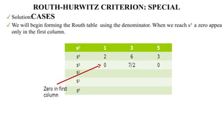
Solution:
We will beginforming the Routh table using the denominator. When we reach s3
a zero appear
only in the first column.
ROUTH-HURWITZ CRITERION: SPECIAL
CASES
150.
If there iszero in the first column we cannot check the sign changes in the first column
because zero does not have ‘+’ or ‘-’.
A solution to this problem is to change 0 into epsilon (ε).
ROUTH-HURWITZ CRITERION: SPECIAL
CASES
151.
We will thencalculate the determinant for the next s values using the
epsilon.
ROUTH-HURWITZ CRITERION: SPECIAL
CASES
152.
If we allthe columns and rows in the Routh table we will get
ROUTH-HURWITZ CRITERION: SPECIAL
CASES
153.
We can findthe number of poles on the right half plane based on the sign
changes in the first column. We can assume ε as ‘+’ or ‘-’
ROUTH-HURWITZ CRITERION: SPECIAL
CASES
154.
There are twosign changes so there are two poles on the right half plane. Thus
the system is unstable.
ROUTH-HURWITZ CRITERION: SPECIAL
CASES
155.
Entire row iszero
the method to solve a Routh table with zeros in entire row is different than
only zero in first column.
When a Routh table has entire row of zeros, the poles could be in the right
half plane, or the left half plane or on the jω axis.
ROUTH-HURWITZ CRITERION: SPECIAL
CASES
Example
Determine the number of right-half-lane poles in the closed-loop transfer
function
We can reducethe number in each
row
ROUTH-HURWITZ CRITERION: SPECIAL
CASES
158.
We stop atthe third row since the entire row consists of zeros.
When this happens, we need to do the following procedure.
ROUTH-HURWITZ CRITERION: SPECIAL
CASES
159.
Return to therow immediately above the row of zeros and form the polynomial.
The polynomial formed is
P ( s) = s4
+ 6s2
+ 8
ROUTH-HURWITZ CRITERION: SPECIAL
CASES
160.
Next we differentiatethe polynomial with respect to s and obtain
We use the coefficient above to replace the row of zeros.
The remainder of the table is formed in a straightforward manner.
ROUTH-HURWITZ CRITERION: SPECIAL
CASES
161.
The Routh tablewhen we change zeros with new values
ROUTH-HURWITZ CRITERION: SPECIAL
CASES
162.
Solve for theremainder of the Routh table
There are no sign changes, so there are no poles on the right half
plane. The system is stable.
ROUTH-HURWITZ CRITERION: SPECIAL
CASES
163.
Example 4 –special case
ROUTH-HURWITZ CRITERION: SPECIAL
CASES
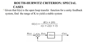
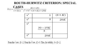
164.
Given that G(s)is the open loop transfer function for a unity feedback
system, find the range of K to yield a stable system
ROUTH-HURWITZ CRITERION: SPECIAL
CASES


![STEPS TO DRAW POLAR PLOT
• Step 1: Determine the T.F G(s)
• Step 2: Put s=jω in the G(s)
• Step 3: At ω=0 & ω=∞ find by &
• Step 4: Rationalize the function G(jω) and separate the real and imaginary parts
• Step 5: Put Re [G(jω) ]=0, determine the frequency at which plot intersects the Im axis and calculate
intersection value by putting the above calculated frequency in G(jω)
• Step 7: Put Im [G(jω) ]=0, determine the frequency at which plot intersects the real axis and
calculate intersection value by putting the above calculated frequency in G(jω)
• Step 8: Sketch the Polar Plot with the help of above information](https://image.slidesharecdn.com/cstemplate-ppt-250408074557-3f805e2a/85/control-systems-template-ppt-pptx-Control-systems-100-320.jpg)


![Type 0 system
• Step 4: Separate the real and Im part of G(jω)
• Step 5: Put Re [G(jω)]=0](https://image.slidesharecdn.com/cstemplate-ppt-250408074557-3f805e2a/85/control-systems-template-ppt-pptx-Control-systems-103-320.jpg)
![Type 0 system
• Step 6: Put Im [G(jω)]=0](https://image.slidesharecdn.com/cstemplate-ppt-250408074557-3f805e2a/85/control-systems-template-ppt-pptx-Control-systems-104-320.jpg)


![Type 1 system
• Step 4: Separate the real and Im part of G(jω)
• Step 5: Put Re [G(jω)]=0](https://image.slidesharecdn.com/cstemplate-ppt-250408074557-3f805e2a/85/control-systems-template-ppt-pptx-Control-systems-107-320.jpg)
![Type 1 system
• Step 6: Put Im [G(jω)]=0](https://image.slidesharecdn.com/cstemplate-ppt-250408074557-3f805e2a/85/control-systems-template-ppt-pptx-Control-systems-108-320.jpg)


![• Step 4: Separate the real and Im part
of G(jω)
By: P.T.KRISHNA SAI, EEE, DIET.
Step 5: Put Im [G(jω)]=0](https://image.slidesharecdn.com/cstemplate-ppt-250408074557-3f805e2a/85/control-systems-template-ppt-pptx-Control-systems-112-320.jpg)