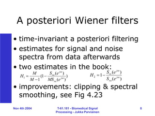
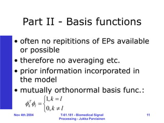
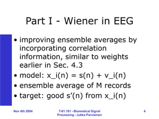
This document discusses Wiener filtering and basis functions for biomedical signal processing. It covers using a Wiener filter to optimally remove noise from EEG signals by incorporating correlation information [1]. It also discusses modeling signals using mutually orthonormal basis functions like Fourier series to analyze single-trial data when repetitions are not available [2]. Limitations of these approaches are noted, such as assumptions of signal stationarity that may not always hold [3].
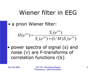
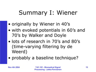
![Nov 4th 2004 T-61.181 - Biomedical Signal
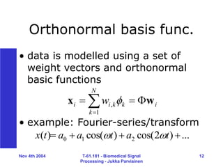
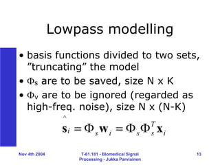
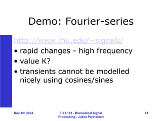
Processing - Jukka Parviainen
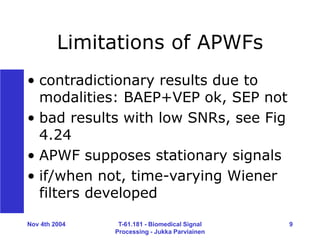
7
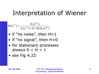
Wiener in theory
• design H(z), so that mean-square
error E[(s(n)-s’(n))^2] minimized
• Wiener-Hopf equations of
noncausal IIR filter lead to H(ej )
• filter gain 0 < H < 1 implies
underestimation (bias)
• bias/variance dilemma](https://image.slidesharecdn.com/eeg2004-240202072255-ec67b193/85/WEINER-FILTERING-AND-BASIS-FUNCTIONS-ppt-7-320.jpg)