This document summarizes key concepts from a chapter on probability, including experimental probability, relative frequency, and examples. It defines an experiment as an activity that produces observed and recorded data. Relative frequency is comparing the number of times an outcome occurs to the total number of observations. Experimental probability is the likelihood an event will occur, calculated by the number of favorable outcomes over the total possible outcomes. Examples are provided to demonstrate calculating experimental probability from survey results and finding the probability of an event based on relative areas. The homework assignment is to complete problems 1 through 20 on page 152.

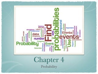
1. Chapter 4
Probability

2. SECTION 4-1
Experiments and Probabilities

3. Essential Questions
How do you collect data with experiments?
How do you use data to find experimental
probabilities?
Where you’ll see this:
Music, market research, games, statistics, probability

4. Vocabulary
1. Experiment:
2. Relative Frequency:
3. Experimental Probability:

5. Vocabulary
1. Experiment: An activity used to produce data that is
observed and recorded
2. Relative Frequency:
3. Experimental Probability:

6. Vocabulary
1. Experiment: An activity used to produce data that is
observed and recorded
2. Relative Frequency: Comparing the number of times an
outcome occurs to the total number of observations
3. Experimental Probability:

7. Vocabulary
1. Experiment: An activity used to produce data that is
observed and recorded
2. Relative Frequency: Comparing the number of times an
outcome occurs to the total number of observations
3. Experimental Probability: The likelihood an event (E) is
going to occur

8. Vocabulary
1. Experiment: An activity used to produce data that is
observed and recorded
2. Relative Frequency: Comparing the number of times an
outcome occurs to the total number of observations
3. Experimental Probability: The likelihood an event (E) is
going to occur
Number of favorable outcomes
P( E ) =
Total number of possible outcomes

9. Activity
Complete the activity from page 150: Flipping a coin

10. Activity
Complete the activity from page 150: Flipping a coin
Number of Tails
Number of Heads

11. Activity
Complete the activity from page 150: Flipping a coin
Number of Tails
Number of Heads
P(Tails) = ?

12. Example 1
Maggie Brann gave samples of a new lipstick and asked the
women who received the samples to rate the lipstick
according to certain standards of appeal. The results of the
survey are below:
Scores 50-59 60-69 70-79 80-89 90-99
Frequency 1 4 2 6 2
What is the experimental probability that a woman who
received a lipstick gave it a rating of at least 80?

13. Example 1
Maggie Brann gave samples of a new lipstick and asked the
women who received the samples to rate the lipstick
according to certain standards of appeal. The results of the
survey are below:
Scores 50-59 60-69 70-79 80-89 90-99
Frequency 1 4 2 6 2
What is the experimental probability that a woman who
received a lipstick gave it a rating of at least 80?
P(Score ≥ 80)

14. Example 1
Maggie Brann gave samples of a new lipstick and asked the
women who received the samples to rate the lipstick
according to certain standards of appeal. The results of the
survey are below:
Scores 50-59 60-69 70-79 80-89 90-99
Frequency 1 4 2 6 2
What is the experimental probability that a woman who
received a lipstick gave it a rating of at least 80?
6+2
P(Score ≥ 80) =
15

15. Example 1
Maggie Brann gave samples of a new lipstick and asked the
women who received the samples to rate the lipstick
according to certain standards of appeal. The results of the
survey are below:
Scores 50-59 60-69 70-79 80-89 90-99
Frequency 1 4 2 6 2
What is the experimental probability that a woman who
received a lipstick gave it a rating of at least 80?
6+2 8
P(Score ≥ 80) = =
15 15

16. Example 1
Maggie Brann gave samples of a new lipstick and asked the
women who received the samples to rate the lipstick
according to certain standards of appeal. The results of the
survey are below:
Scores 50-59 60-69 70-79 80-89 90-99
Frequency 1 4 2 6 2
What is the experimental probability that a woman who
received a lipstick gave it a rating of at least 80?
6+2 8
P(Score ≥ 80) = = = 53 1 3 %
15 15

17. Example 2
What is the probability that a dart thrown at this
dartboard will land in the bull’s-eye? The radius of the
smallest circle is 2 cm, and each band is also 2 cm wide.

18. Example 2
What is the probability that a dart thrown at this
dartboard will land in the bull’s-eye? The radius of the
smallest circle is 2 cm, and each band is also 2 cm wide.
P(Bull's-eye)

19. Example 2
What is the probability that a dart thrown at this
dartboard will land in the bull’s-eye? The radius of the
smallest circle is 2 cm, and each band is also 2 cm wide.
P(Bull's-eye)
Area of smallest circle
=
Area of largest circle

20. Example 2
What is the probability that a dart thrown at this
dartboard will land in the bull’s-eye? The radius of the
smallest circle is 2 cm, and each band is also 2 cm wide.
P(Bull's-eye)
Area of smallest circle
=
Area of largest circle
2
π (2)
= 2
π (6)

21. Example 2
What is the probability that a dart thrown at this
dartboard will land in the bull’s-eye? The radius of the
smallest circle is 2 cm, and each band is also 2 cm wide.
P(Bull's-eye)
Area of smallest circle
=
Area of largest circle
π (2) = 4
2
=
π (6) 2 36

22. Example 2
What is the probability that a dart thrown at this
dartboard will land in the bull’s-eye? The radius of the
smallest circle is 2 cm, and each band is also 2 cm wide.
P(Bull's-eye)
Area of smallest circle
=
Area of largest circle
π (2) = 4 = 1
2
=
π (6) 2 36 9

23. Example 2
What is the probability that a dart thrown at this
dartboard will land in the bull’s-eye? The radius of the
smallest circle is 2 cm, and each band is also 2 cm wide.
P(Bull's-eye)
Area of smallest circle
=
Area of largest circle
π (2) = 4 = 1
2
=
π (6) 2 36 9
= 11 1 9 %

24. Example 2
What is the probability that a dart thrown at this
dartboard will land in the bull’s-eye? The radius of the
smallest circle is 2 cm, and each band is also 2 cm wide.
P(Bull's-eye)
Area of smallest circle
=
Area of largest circle
π (2) = 4 = 1
2
=
π (6) 2 36 9
= 11 1 9 %
Favorable area
P(Area) =
Total area

25. Homework

26. Homework
p. 152 #1-20
“Liberty means responsibility. That is why most men dread it.”
- George Bernard Shaw