The document discusses term weighting and similarity measures in information retrieval. It explains the significance of term-document matrices, binary and non-binary weights, as well as term frequency (tf), inverse document frequency (idf), and tf*idf weighting techniques to improve document relevance ranking. Additionally, it covers similarity measures such as Euclidean distance, inner product, and cosine similarity for evaluating the relevance between documents and queries.

1. Chapter Three
Term weighting and
similarity measures
1

2. 2
term-document matrix
• Documents and queries are represented as vectors or “bags of
words” (BOW) in a term-document matrix.
• An entry in the matrix corresponds to the “weight” of a term in
the document
–The weight of terms (wij) may be a binary weight or Non-binary weight
. wij is zero means the term doesn’t exist in the document.
T1 T2 …. Tt
D1 w11 w21 … wt1
D2 w12 w22 … wt2
: : : :
: : : :
Dn w1n w2n … wtn









0
else
0
0
if
1
ij
ij
ij
freq
freq
W


3. Binary Weights
• Only the presence (1) or
absence (0) of a term is
included in the vector
• Binary formula gives every
word that appears in a
document equal relevance.
• It can be useful when
frequency is not important.
• Binary Weights Formula:
docs t1 t2 t3
D1 1 0 1
D2 1 0 0
D3 0 1 1
D4 1 0 0
D5 1 1 1
D6 1 1 0
D7 0 1 0
D8 0 1 0
D9 0 0 1
D10 0 1 1
D11 1 0 1








0
if
0
0
if
1
ij
ij
ij
freq
freq
freq

4. 4
Why use term weighting?
• Binary weights are too limiting.
– Terms are either present or absent.
– Not allow to order documents according to their level of
relevance for a given query
• Non-binary weights allow to model partial matching.
– Partial matching allows retrieval of documents that
approximate the query.
• Term-weighting helps to apply best matching that
improves quality of answer set.
– Term weighting enables ranking of retrieved documents; such
that best matching documents are ordered at the top as they
are more relevant than others.

5. Term Weighting: Term Frequency (TF)
• TF (term frequency) - Count the number of
times term occurs in document.
fij = frequency of term i in document j
• The more times a term t occurs in
document d the more likely it is that t is
relevant to the document, i.e. more
indicative of the topic..
– If used alone, it favors common words and
long documents.
– It gives too much credit to words that appears
more frequently.
• May want to normalize term frequency (tf)
docs t1 t2 t3
D1 2 0 3
D2 1 0 0
D3 0 4 7
D4 3 0 0
D5 1 6 3
D6 3 5 0
D7 0 8 0
D8 0 10 0
D9 0 0 1
D10 0 3 5
D11 4 0 1

6. 6
Document Normalization
• Long documents have an unfair
advantage:
– They use a lot of terms
• So they get more matches than short
documents
– And they use the same words repeatedly
• So they have much higher term frequencies
• Normalization seeks to remove these
effects:
– Related somehow to maximum term frequency.
– But also sensitive to the number of terms.
• If we don’t normalize short documents
may not be recognized as relevant.

7. Problems with term frequency
• Need a mechanism for decreasing the effect of terms that
occur too often in the collection to be meaningful for
relevance/meaning determination
• Scale down the weight of terms with high collection
frequency
– Reduce the tf weight of a term by a factor that grows
with the collection frequency
• More common for this purpose is document frequency
– how many documents in the collection contain the term
7
• The example shows that collection
frequency and document frequency
behaves differently

8. 8
Document Frequency
• It is defined to be the number of documents in the
collection that contain a term
DF = document frequency
– Count the frequency considering the whole
collection of documents.
– Less frequently a term appears in the whole
collection, the more discriminating it is.
dfi (document frequency of term i)
= number of documents containing term i

9. Inverse Document Frequency (IDF)
• IDF measures rarity of the term in collection. The IDF is a
measure of the general importance of the term
– Inverts the document frequency.
• It reduces the weight of terms that occur very frequently
in the collection and increases the weight of terms that
occur rarely.
– Gives full weight to terms that occur in one document
only.
– Gives zero weight to terms that occur in all documents.
– Terms that appear in many different documents are less
indicative of overall topic.
idfi = inverse document frequency of term i, where N: total
number of documents
9
)
/
(
log2 i
i df
N
idf 

10. 10
Inverse Document Frequency
• IDF provides high values for rare words and low values
for common words.
• IDF is an indication of a term’s discrimination power.
– Log used to dampen the effect relative to tf.
– Make the difference between Document frequency vs. corpus
frequency ?
• Example: given a collection of 1000 documents and
document frequency, compute IDF for each word?
Word N DF IDF
the 1000 1000 0
some 1000 100 3.322
car 1000 10 6.644
merge 1000 1 9.966

11. TF*IDF Weighting
• A good weight must take into account two effects:
– Quantification of intra-document contents (similarity)
• tf factor, the term frequency within a document
– Quantification of inter-documents separation
(dissimilarity)
• idf factor, the inverse document frequency
• As a result of which the most widely used term-
weighting by IR systems is tf*idf weighting technique:
wij = tfij idfi = tfij * log2 (N/ dfi)
• A term occurring frequently in the document but rarely in
the rest of the collection is given high weight.
– The tf*idf value for a term will always be greater than or equal
to zero. 11

12. TF*IDF weighting
• When does TF*IDF registers a high weight? when a term t
occurs many times within a small number of documents
– Highest tf*idf for a term shows a term has a high term frequency
(in the given document) and a low document frequency (in the
whole collection of documents);
– the weights hence tend to filter out common terms.
– Thus lending high discriminating power to those documents
• Lower TF*IDF is registered when the term occurs fewer
times in a document, or occurs in many documents
– Thus contribution a less marked relevance signal
• Lowest TF*IDF is registered when the term occurs in
almost all documents

13. Computing TF-IDF: An Example
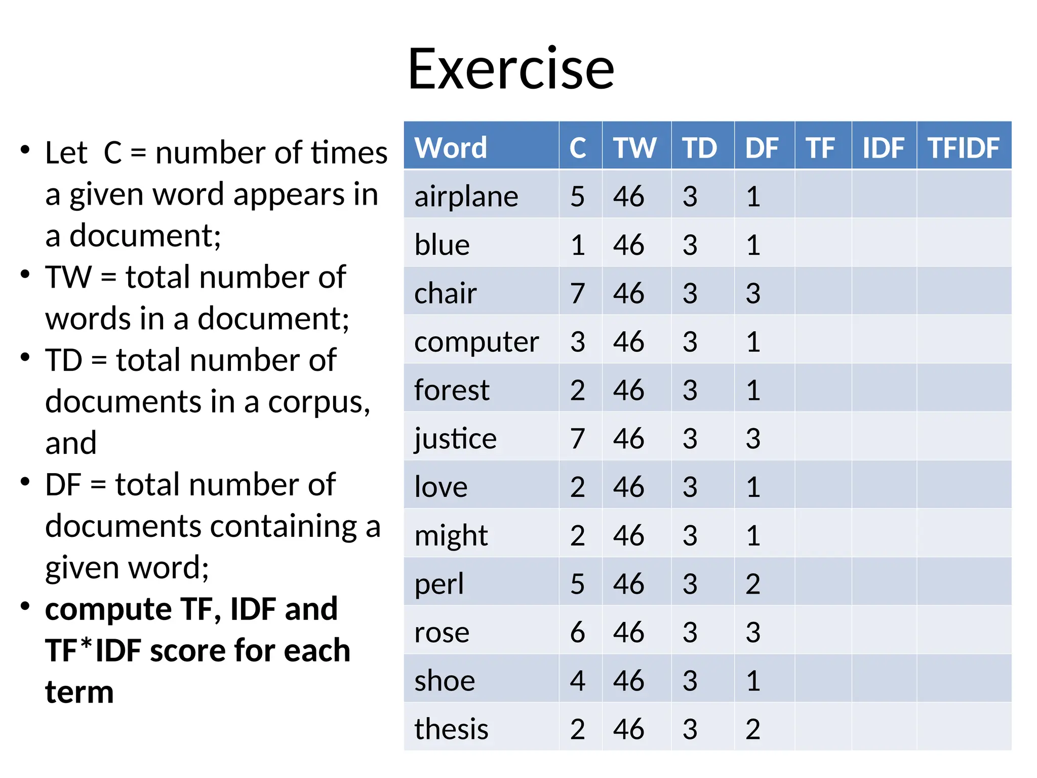
• Assume collection contains 10,000 documents and statistical
analysis shows that document frequencies (DF) of three
terms are: A(50), B(1300), C(250). And also term
frequencies (TF) of these terms are: A(3), B(2), C(1).
Compute TF*IDF for each term?
A: tf = 3/3=1.00; idf = log2(10000/50) = 7.644; tf*idf = 7.644
B: tf = 2/3=0.67; idf = log2(10000/1300) = 2.943; tf*idf = 1.962
C: tf = 1/3=0.33; idf = log2(10000/250) = 5.322; tf*idf = 1.774
• Query is also treated as a short document and also tf-idf
weighted.
wij = (0.5 + [0.5*tfij ])* log2 (N/ dfi)
13

14. More Example
• Consider a document containing 100 words
wherein the word computer appears 3 times.
Now, assume we have 10, 000, 000 documents
and computer appears in 1, 000 of these.
– The term frequency (TF) for computer :
3/100 = 0.03
– The inverse document frequency is
log2(10,000,000 / 1,000) = 13.228
– The TF*IDF score is the product of these frequencies:
0.03 * 13.228 = 0.39684
14

15. Exercise
15
• Let C = number of times
a given word appears in
a document;
• TW = total number of
words in a document;
• TD = total number of
documents in a corpus,
and
• DF = total number of
documents containing a
given word;
• compute TF, IDF and
TF*IDF score for each
term
Word C TW TD DF TF IDF TFIDF
airplane 5 46 3 1
blue 1 46 3 1
chair 7 46 3 3
computer 3 46 3 1
forest 2 46 3 1
justice 7 46 3 3
love 2 46 3 1
might 2 46 3 1
perl 5 46 3 2
rose 6 46 3 3
shoe 4 46 3 1
thesis 2 46 3 2

16. Similarity Measure
• We now have vectors for all documents in the
collection, a vector for the query, how to
compute similarity?
• A similarity measure is a function that
computes the degree of similarity or distance
between document vector and query vector.
• Using a similarity measure between the query
and each document:
– It is possible to rank the retrieved
documents in the order of presumed
relevance.
– It is possible to enforce a certain beginning
so that the size of the retrieved set can be
controlled.
16

t3
t1
t2
D1
D2
Q


17. Similarity/Dissimilarity Measures
•Euclidean distance
–It is the most common similarity measure. Euclidean
distance examines the root of square differences between
coordinates of a pair of document and query terms.
• Dot product
–The dot product is also known as the scalar product or
inner product
–the dot product is defined as the product of the
magnitudes of query and document vectors
• Cosine similarity (or normalized inner product)
–It projects document and query vectors into a term space
and calculate the cosine angle between these.
17

18. Euclidean distance
• Similarity between vectors for the document di and query
q can be computed as:
sim(dj,q) = |dj – q| =
where wij is the weight of term i in document j and wiq
is the weight of term i in the query
• Example: Determine the Euclidean distance between
the document 1 vector (0, 3, 2, 1, 10) and query vector
(2, 7, 1, 0, 0). 0 means corresponding term not found in
document or query



n
i
iq
ij w
w
1
2
)
(
18
05
.
11
)
0
10
(
)
0
1
(
)
1
2
(
)
7
3
(
)
2
0
( 2
2
2
2
2












19. 19
Dissimilarity Measures
• Euclidean distance is generalized to the popular
dissimilarity measure called: Minkowski distance:
where X = (x1, x2, …, xn) and Y = (y1, y2, …, yn) are two n-
dimensional data objects; n is size of vector attributes of
the data object; q= 1,2,3,…
m
n
i
m
iq
ij
iq
ij w
w
w
w
Dis 



1
)
(
)
,
(

20. Inner Product
• Similarity between vectors for the document di and query q
can be computed as the vector inner product:
sim(dj,q) = dj•q = wij · wiq
where wij is the weight of term i in document j and wiq is
the weight of term i in the query q
• For binary vectors, the inner product is the number of
matched query terms in the document (size of intersection).
• For weighted term vectors, it is the sum of the products of
the weights of the matched terms.


n
i 1
20

21. Inner Product -- Examples
Retrieval Database Architecture
D1 2 3 5
D2 3 7 1
Q 1 0 2
• Given the following term-document matrix, using
inner product which document is more relevant for
the query Q?
• sim(D1 , Q) = 2*1 + 3*0 + 5*2 = 12
• sim(D2 , Q) = 3*1 + 7*0 + 1*2 = 5

22. Cosine similarity
• Measures similarity between d1 and d2 captured by the
cosine of the angle x between them.
• The denominator involves the lengths of the vectors
• So the cosine measure is also known as the normalized
inner product









n
i q
i
n
i j
i
n
i q
i
j
i
j
j
j
w
w
w
w
q
d
q
d
q
d
sim
1
2
,
1
2
,
1 ,
,
)
,
( 



 

n
i j
i
j w
d 1
2
,
Length


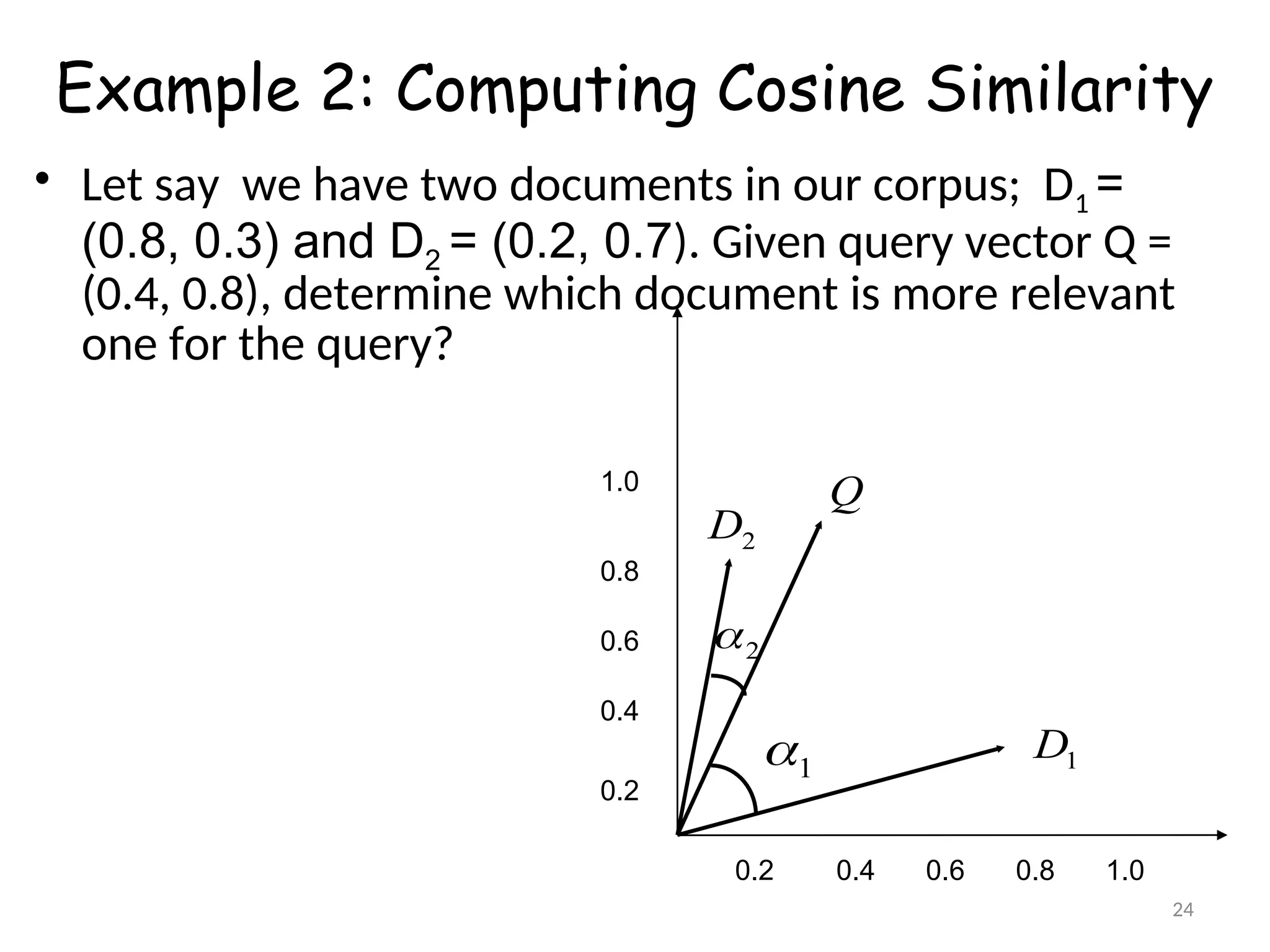
23. Example 1: Computing Cosine Similarity
98
.
0
42
.
0
64
.
0
]
)
7
.
0
(
)
2
.
0
[(
*
]
)
8
.
0
(
)
4
.
0
[(
)
7
.
0
*
8
.
0
(
)
2
.
0
*
4
.
0
(
)
,
(
2
2
2
2
2






D
Q
sim
• Let say we have query vector Q = (0.4, 0.8); and also
document D1 = (0.2, 0.7). Compute their similarity
using cosine?

24. 24
Example 2: Computing Cosine Similarity
2

1
 1
D
Q
2
D
1.0
0.8
0.6
0.8
0.4
0.6
0.4 1.0
0.2
0.2
• Let say we have two documents in our corpus; D1 =
(0.8, 0.3) and D2 = (0.2, 0.7). Given query vector Q =
(0.4, 0.8), determine which document is more relevant
one for the query?

25. Example
• Given three documents; D1, D2 and D3 with the
corresponding TFIDF weight, Which documents are more
similar using the three similarity measurement?
25
Terms D1 D2 D3
affection 0.996 0.993 0.847
Jealous 0.087 0.120 0.466
gossip 0.017 0.000 0.254