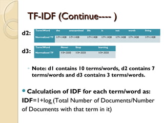
Downloaded 24 times
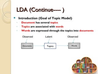
![TF-IDF (Continue---- )TF-IDF (Continue---- )
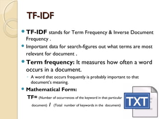
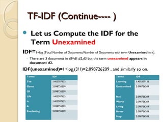
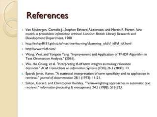
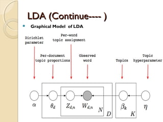
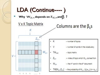
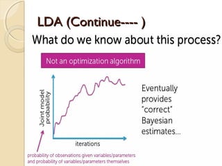
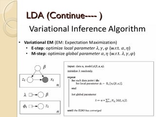
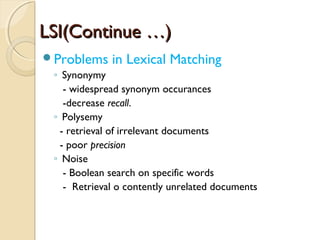
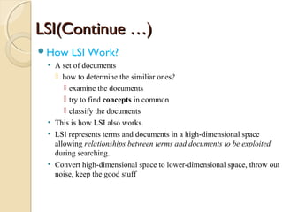
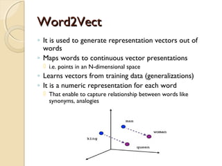
Vector Space Model-Cosine Similarity
◦ For each document we derive a vector
◦ Set of documents in a collection is viewed as a set of
vectors in a vector space.
◦ Each term will have its own axis
Formula: To find similarity b/w any two documents
Cosine Similarity (d1, d2) = Dot product(d1, d2) / ||d1|| * ||d2||
Dot product (d1,d2) = d1[0] * d2[0] + d1[1] * d2[1] * … * d1[n] * d2[n]
||d1|| = square root(d1[0]2
+ d1[1]2
+ ... + d1[n]2
)
||d2|| = square root(d2[0]2
+ d2[1]2
+ ... + d2[n]2
)](https://image.slidesharecdn.com/dataminingtechniques-180124192518/85/Data-mining-techniques-8-320.jpg)
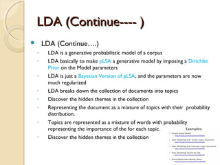
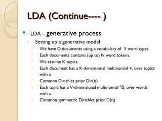
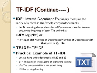
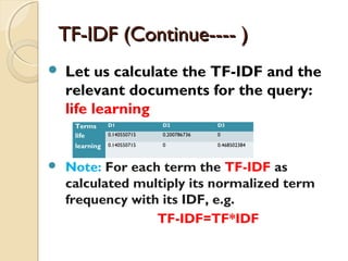
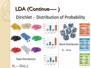
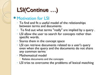
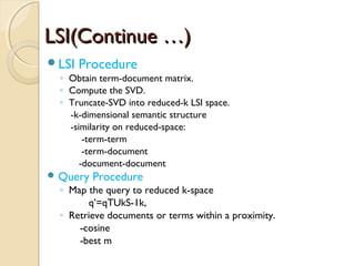
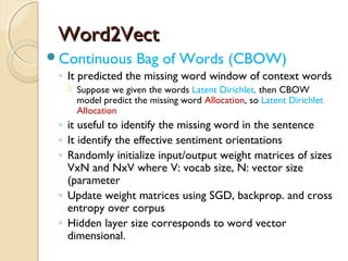
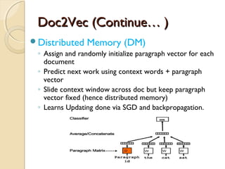
![LDA (Continue---- )LDA (Continue---- )
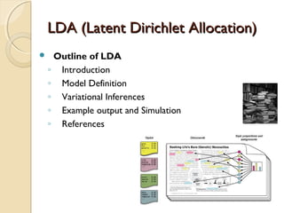
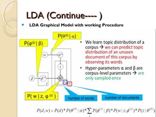
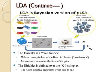
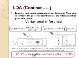
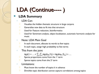
The Generative process
◦ For topic topic k=1…..K do
-Draw a word-distribution(multinomial) Βk Dir( )∼ ɳ
◦ For each document d=1……D do
- Draw a topic-distribution (multinomial)θd Dir( )∼ α
- For each word Wd,n:
◦ - Draw a topic Zd,n Mult(∼ Փd) with Zd,n€ [1…K]
◦ - Draw a word Wd,n Mult( Z∼ β d,n )](https://image.slidesharecdn.com/dataminingtechniques-180124192518/85/Data-mining-techniques-19-320.jpg)
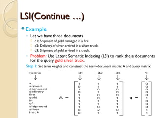
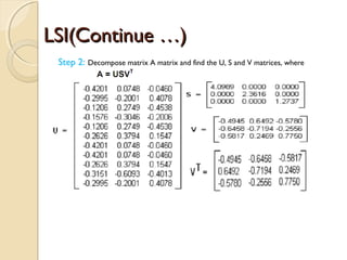
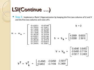
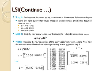

The document explains data mining techniques focused on tf-idf (term frequency-inverse document frequency) and LDA (latent Dirichlet allocation), which are used to quantify the relevance of terms in documents and to discover hidden themes in large corpora, respectively. It covers the mathematical foundations, applications, and limitations of tf-idf and LDA, including examples of how to compute these models and their use in topics like text analysis and semantic understanding. The document also discusses latent semantic indexing (LSI) to address issues like synonymy and polysemy in lexical matching.


![谷歌留痕技术教程[ 𝙩𝙤𝙥 𝟮𝟯𝟯. 𝙘 𝙤𝙢 ]](https://cdn.slidesharecdn.com/ss_thumbnails/top233-260130173900-2eb784f9-thumbnail.jpg?width=640&height=640&fit=bounds)


