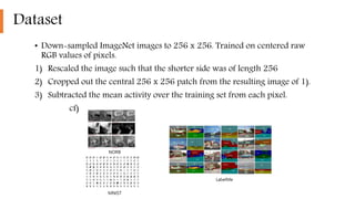
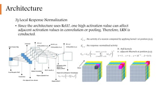
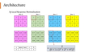
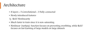
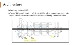
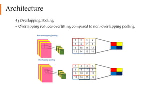
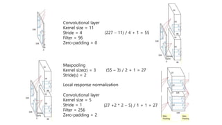
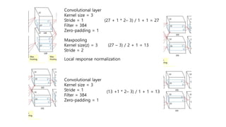
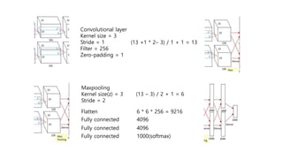
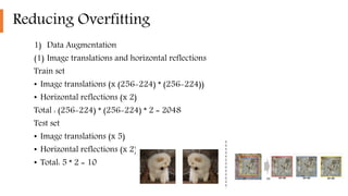
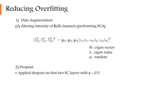
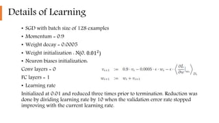
1) The document describes a study that trained one of the largest convolutional neural networks on the ImageNet dataset. 2) It implemented highly optimized GPU training of large CNNs on high resolution images and introduced features like ReLU, local response normalization, and overlapping pooling to improve performance and reduce overfitting. 3) The network architecture consisted of 5 convolutional layers and 3 fully-connected layers and was trained on two GPUs with techniques like dropout and data augmentation to reduce overfitting.

1. ImageNet Classification with Deep
Convolutional Neural Networks
신우철

2. Introduction
1. Trained one of the largest CNN on ImageNet data. The advantages of CNN
are 1) CNN’s prior knowledge, which are stationarity of statistics and
locality of pixel dependencies, 2) its easiness to be controlled, varying its
depth and breath, contributing to fewer parameters and easier training.
2. Implemented highly-optimized GPU implementation to facilitate the
training of large CNNs on high resolution images.
3. Introduced new features to improve performance, reduce training time,
and prevent overfitting.

3. Dataset
• Down-sampled ImageNet images to 256 x 256. Trained on centered raw
RGB values of pixels.
1) Rescaled the image such that the shorter side was of length 256
2) Cropped out the central 256 x 256 patch from the resulting image of 1).
3) Subtracted the mean activity over the training set from each pixel.
cf)
NORB
MNIST
LabelMe

4. Architecture
• 8 layers = 5 Convolutional + 3 Fully-connected
• Newly introduced features
1) ReLU Nonlinearity
• Much faster to train since it is non-saturating
• Nonlinear |tanh(x)| function focuses on preventing overfitting, while ReLU
focuses on fast learning of large models on large datasets

5. Architecture
2) Training on two GPUs
• Cross-GPU parallelization, while the GPUs only communicate in certain
layers. This is to tune the amount of computation by communication.

6. Architecture
3) Local Response Normalization
• Since the architecture uses ReLU, one high activation value can affect
adjacent activation values in convolution or pooling. Therefore, LRN is
conducted.
filter
: the activity of a neuron computed by applying kernel i at position (x,y)
: the response-normalized activity
N : #all kernels
n : adjacent #kernels at position (x,y)

7. Architecture
3) Local Response Normalization
filter 0 filter 1 filter 2 filter 3
1 2 3 1 2 1 2 1 2 4 2 1
4 5 6 2 3 2 3 2 3 5 2 1
7 8 9 3 4 3 4 3 4 2 2 4
0.50 0.25 0.30 0.17 0.22 0.07 0.10 0.11 0.33 0.20 0.40 0.20
0.20 0.15 0.15 0.07 0.08 0.04 0.08 0.12 0.21 0.15 0.25 0.10
0.12 0.10 0.10 0.04 0.04 0.03 0.14 0.10 0.10 0.10 0.15 0.13
k alpha beta n N
0 1 1 2 4
=
2
{0 + 1 x 12 + 22 + 42 }1

8. Architecture
4) Overlapping Pooling
• Overlapping reduces overfitting compared to non-overlapping pooling.

9. Architecture
5) Overall architecture

10. Convolutional layer
Kernel size = 11
Stride = 4
Filter = 96
Zero-padding = 0
(227 – 11) / 4 + 1 = 55
Maxpooling
Kernel size(z) = 3
Stride(s) = 2
Convolutional layer
Kernel size = 5
Stride = 1
Filter = 256
Zero-padding = 2
(55 – 3) / 2 + 1 = 27
(27 +2 * 2 – 5) / 1 + 1 = 27
Local response normalization

11. Convolutional layer
Kernel size = 3
Stride = 1
Filter = 384
Zero-padding = 1
(27 + 1 * 2– 3) / 1 + 1 = 27
Convolutional layer
Kernel size = 3
Stride = 1
Filter = 384
Zero-padding = 1
(13 +1 * 2– 3) / 1 + 1 = 13
Maxpooling
Kernel size(z) = 3
Stride = 2
(27 – 3) / 2 + 1 = 13
Local response normalization

12. Convolutional layer
Kernel size = 3
Stride = 1
Filter = 256
Zero-padding = 1
(13 +1 * 2– 3) / 1 + 1 = 13
Maxpooling
Kernel size(z) = 3
Stride = 2
(13 – 3) / 2 + 1 = 6
Flatten 6 * 6 * 256 = 9216
Fully connected 4096
Fully connected 4096
Fully connected 1000(softmax)

13. Reducing Overfitting
1) Data Augmentation
(1) Image translations and horizontal reflections
Train set
• Image translations (x (256-224) * (256-224))
• Horizontal reflections (x 2)
Total : (256-224) * (256-224) * 2 = 2048
Test set
• Image translations (x 5)
• Horizontal reflections (x 2)
• Total: 5 * 2 = 10

14. Reducing Overfitting
1) Data Augmentation
(2) Altering intensity of RGB channels (performing PCA)
2) Dropout
• Applied dropout on first two FC layers with p = 0.5
Pi : eigen vector
 : eigen value
 : random
=

15. Details of Learning
• SGD with batch size of 128 examples
• Momentum = 0.9
• Weight decay = 0.0005
• Weight initialization : N(0, 0.012
)
• Neuron biases initialization:
Conv layers = 0
FC layers = 1
• Learning rate
Initialized at 0.01 and reduced three times prior to termination. Reduction was
done by dividing learning rate by 10 when the validation error rate stopped
improving with the current learning rate.

16. Results

17. Results
• Result of restricted connectivity between two GPUs result in specialization.
Kernels on GPU 1 are largely color-agnostic, while kernels on GPU 2 are
largely color-specific.
• Perform kNN at the last 4096-dimensional hidden layer shows that images
are semantically similar.