This document provides an overview of deep learning techniques for image analysis using convolutional neural networks (CNNs). It discusses how CNNs use convolutional filters to extract hierarchical features from images and how techniques like pooling, dropout and residual connections improve CNN performance. Practical examples are given on using CNNs for tasks like object recognition, object detection and semantic segmentation on datasets like MNIST and pretrained models like ResNet-18.

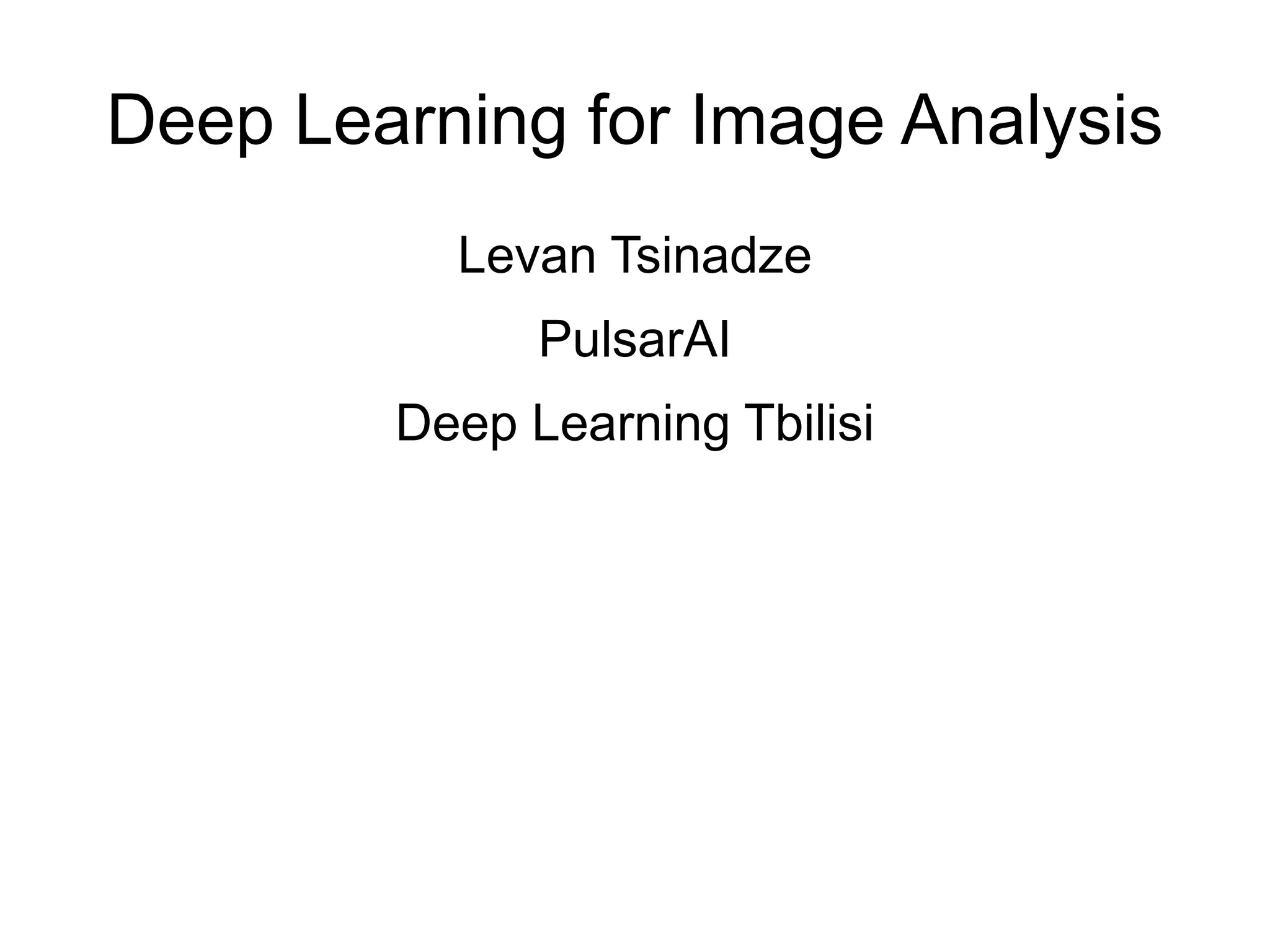
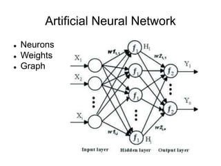
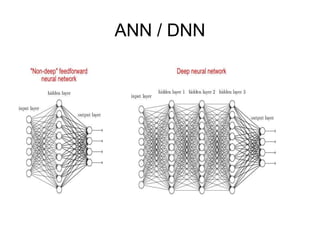
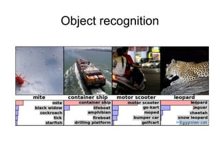
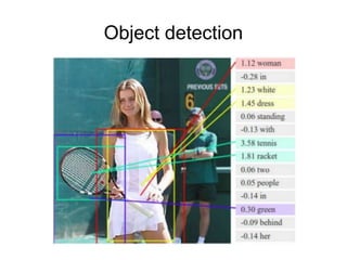
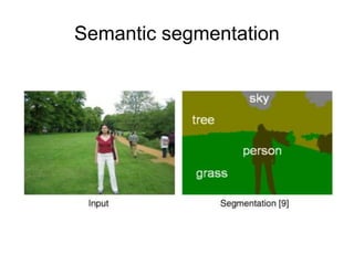
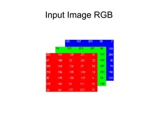
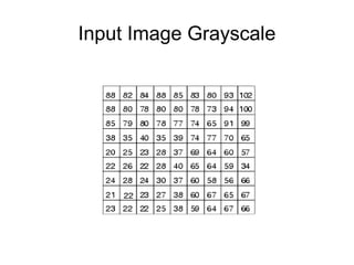
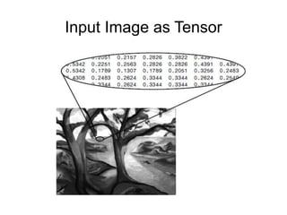
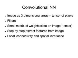
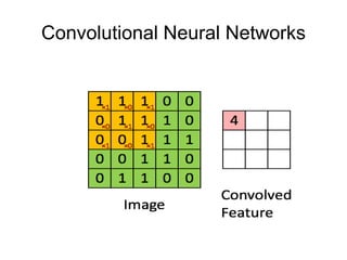
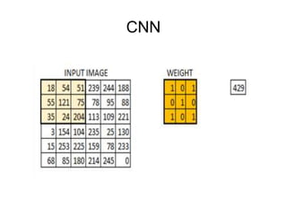
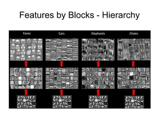
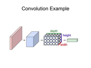
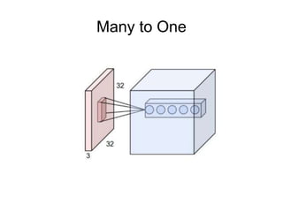
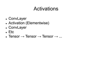
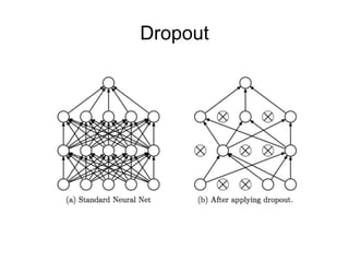
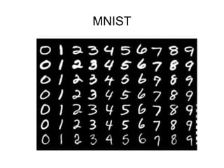
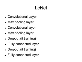
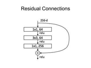
1. Deep Learning for Image Analysis
Levan Tsinadze
PulsarAI
Deep Learning Tbilisi

2. Artificial Neural Network
 Neurons
 Weights
 Graph

3. Neuron

4. Specifications
 Input Layer – Hidden Layers – Output Layer
 “Easy” Functions
 Parallelism (Matrices)

5. ANN / DNN

6. Problems in CV
 Object recognition
 Object detection
 Semantic segmentation

7. Object recognition

8. Object detection

9. Semantic segmentation

10. Hybrid Models – Detect - Recognize

11. Input Image RGB

12. Input Image Grayscale

13. Input Image as Tensor

14. Convolutional NN
 Image as 3 dimensional array – tensor of pixels
 Filters
 Small matrix of weights slide on image (tensor)
 Step by step extract features from image
 Locall connectivity and spatial invariance

15. Convolutional Neural Networks

16. CNN

17. Filter - Input - Output
 Input – tensor
 Output – matrix
 Depth is shrinked

18. Convolutional Block
 Convolutional fiters (often more than one)
 Activation
 Pooling

19. Features by Blocks - Hierarchy

20. Number of Filters
 Input channel – Image Depth (RGB)
 Output channel – Hyper Parameter number of
convolutional filters (kernels)
 Feature Map – Generated Matrix for Each
Patch
 Feature Maps on top of each other

21. Convolution Example

22. Many to One

23. Weight Shearing
 Features map – small amount of weights
 6x6 input 10 features matrices 3x3 each 90
parameters produces 4x4x10 tensor
 224x224x3 to 2048 get 101054464 parameters
 Fully connected layer 6x6x4x4 = 576
 32 Features map
 256 or even 512 or 1024 features map
 Still better presision with less parameters = less
calculation

24. FP – Sparce FFNN

25. Activations
 ConvLayer
 Activation (Elementwise)
 ConvLayer
 Etc
 Tensor → Tensor → Tensor → ...

26. ReLU
 x = x < 0 ? 0 : x or x = max(0, x)
 9:15 – Graph
 Df/Dx = 0 when x = 0
 Easy to Propagate (Forward and Back)
 Easy to See Results

27. ReLU - Watch

28. ReLU - Graph

29. Pooling

30. Pooling Types
 Max-Pooling
 Average – Pooling
 L2-Norm-Poolig

31. Pooling – Down-Sampling

32. Pooling only on Matrices
 Only Matrices
 Pooling for each Channel
 Same Dimensions
 Height Changes
 Width Changes

33. Dropout

34. MNIST

35. LeNet
 Convolutional Layer
 Max pooling layer
 Convolutional layer
 Max pooling layer
 Dropout (if training)
 Fully connected layer
 Dropout (if training)
 Fully connected layer

36. Training Epochs
 Train
 Shuffle
 Train again
 Only on training set
 Avoid local minimum

37. PyTorch
 Dynamic execution
 Imperative
 Object-oriented
 http://pytorch.org/

38. Practical Example

39. Fine-Tuning / Transfer Learning
 Freeze lower layers
 Retrain higher layers
 Small dataset
 Fast training
 Less resources

40. ResNet-18
 Residual connections
 Vanishing gradient
 Very deep convolutional neural network
 Easy architecture
 Eveilable pretrained (On ImageNet) weights

41. Residual Connections

42. Practical Example

43. One / N – Shot Learning
 Retraining problems
 Labeling problems (Letters OK, Numbers OK
Faces NOT OK)
 Features extractors
 Feature Search

44. Embedding Vectors

45. Features Extractor
 Text
 Image
 Features - Vector

46. Faces

47. Image Similarities