Download to read offline


![Space-Variant Image Restoration with Running Sinusoidal Transforms 7
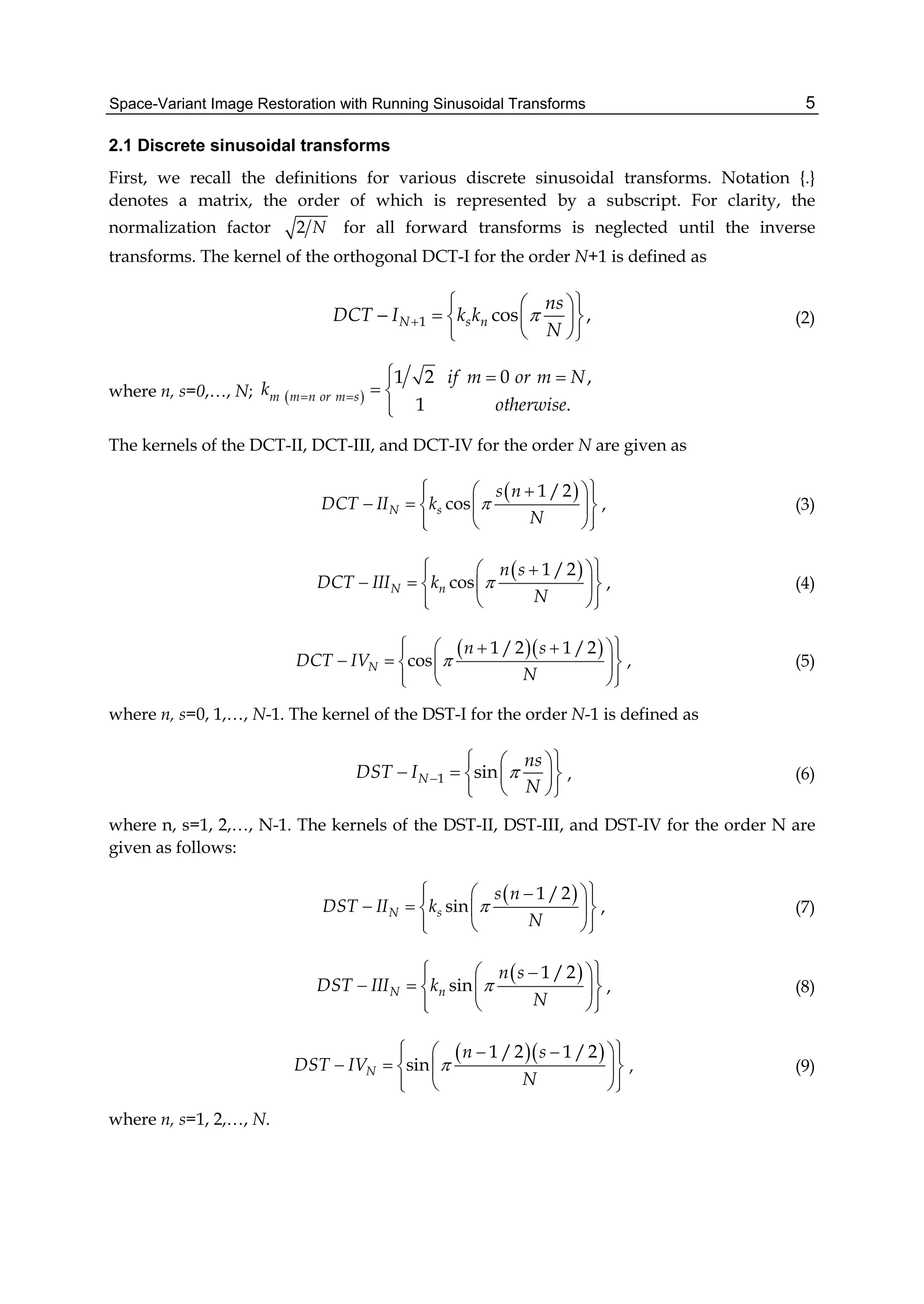
The number of arithmetic operations required for computing the running discrete cosine
transforms at a given window position is evaluated as follows. The SDCT-I for the order
N+1 with N=N1+N2 requires N-1 multiplication operations and 4(N+2) addition operations.
The SDCT-II for the order N with N= N1+ N2+1 requires 2(N-1) multiplication operations
and 2N+5 addition operations. A fast algorithm for the SDCT-III for the order N with N=N1+
N2+1 is based on the recursive equation given in line 3 of Table 1. Next it is useful to
represent the equation as
2
1 1
1
1 /2 1 /2
cos 1 sin
sk k k k
s s s s k N
s s
X X X X x
N N
, (10)
where the array 1
; 0 1 . 1k k
s s k NX X x s , ,.. N is stored in a memory buffer of N
elements. From the property of symmetry of the sine function, sin 1 /2s N
sin 1 /2 , 0,1,...[ /2]N s N s N (here [x/y] is the integer quotient) and Eq. (10), the
number of operations required to compute the DSCT-III can be evaluated as [3/2N]
multiplication operations and 4N addition operations. An additional memory buffer of N
elements is also required. Finally, the SDCT-IV for the order N with N=N1+ N2+1 requires
3N multiplication operations and 3N+2 addition operations.
The number of arithmetic operations required for computing the running discrete sine
transforms at a given window position can be evaluated as follows. The SDST-I for the order
N-1 with N=N1+ N2+1 requires 2(N-1) multiplication operations and 2N addition operations.
However, if N is even, 1 21 11 sin
s
k N k Nf s x x s N in line 5 of Table I is
symmetric on the interval [1, N-1]; that is, f(s)=f(N-s), s=1,..N/2-1. Therefore, only N/2-1
multiplication operations are required to compute this term. The total number of
multiplications is reduced to 3N/2-2. The SDST-II for the order N with N=N1+ N2+1 requires
2(N-1) multiplication operations and 2N+5 addition operations. Taking into account the
property of symmetry of the sine and cosine functions, the SDST-III for the order N with
N=N1+ N2+1 requires 2N multiplications and 4N addition operations. However, if N is even,
the sum 1 21( ) sin 1 /2 1 cos 1 /2
s
k N k Ng s x s N x s N in line 7 of Table I
is symmetric on the interval [1, N]; that is, g(s)=g(N-s+1), s=1,..N/2. Therefore, only N/2
addition operations are required to compute the sum. If N is odd, the sum
1 21 1sin 1 /2 1
s
k N k Np s x s N x in line 7 of Table I is symmetric on the
interval [1, N]; that is, p(s)=p(N-s+1), s=1,..[N/2]. Hence, [N/2] addition operations are
required to compute this sum. So, the total number of additions can be reduced to [7N/2].
Finally, the SDST-IV for the order N with N=N1+ N2+1 requires 3N multiplication operations
and 3N+2 addition operations. The length of a moving window for the proposed algorithms
may be an arbitrary integer.
2.3 Fast inverse algorithms for running signal processing with sinusoidal transforms
The inverse discrete cosine and sine transforms for signal processing in a running window
are performed for computing only the pixel xk of the window. The running signal
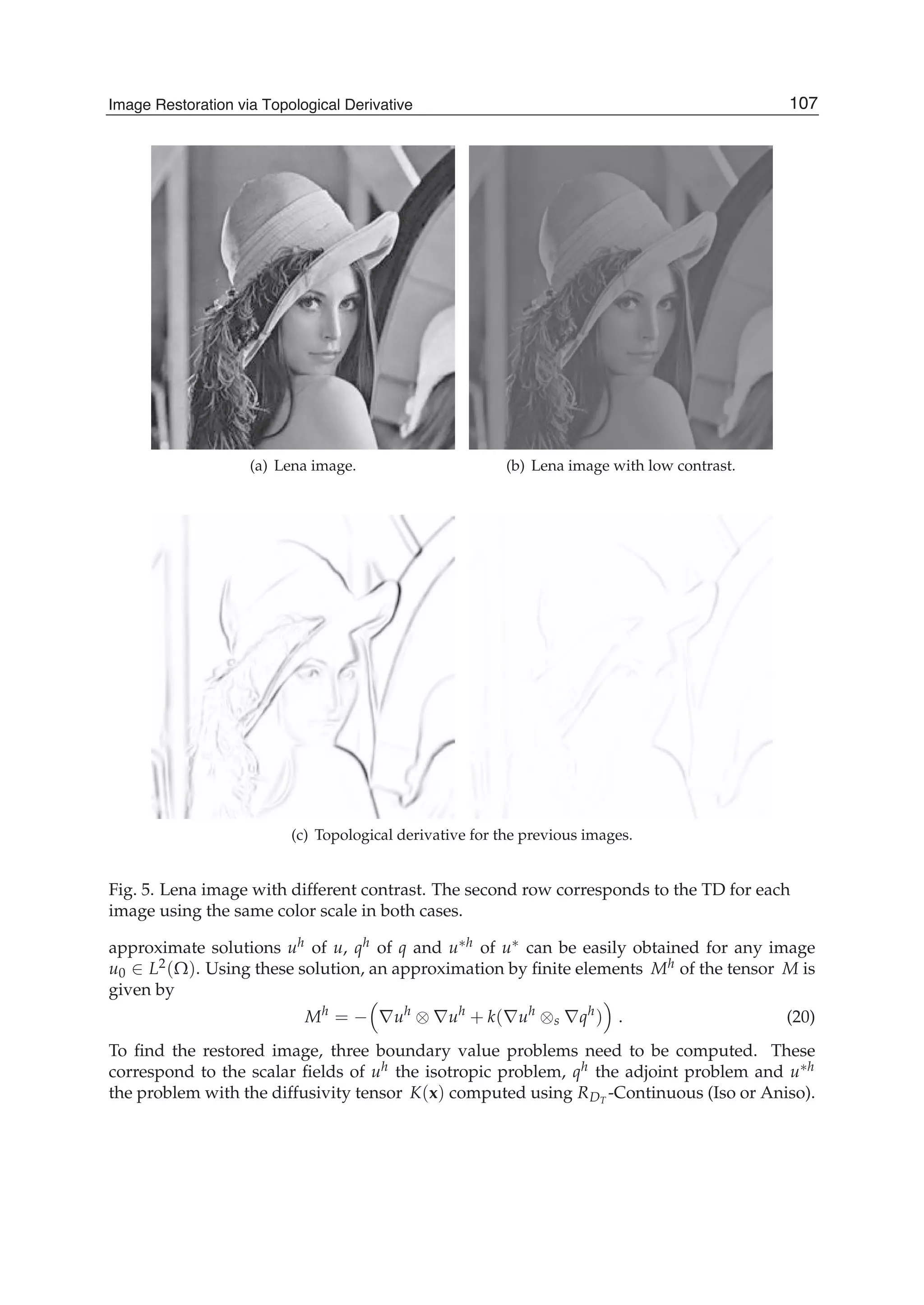
processing can be performed with the use of the SDCT and SDST algorithms.](https://image.slidesharecdn.com/imagerestorationrecentadvancesandapplications-160714160024/75/Image-restoration-recent_advances_and_applications-17-2048.jpg)
![Image Restoration – Recent Advances and Applications8
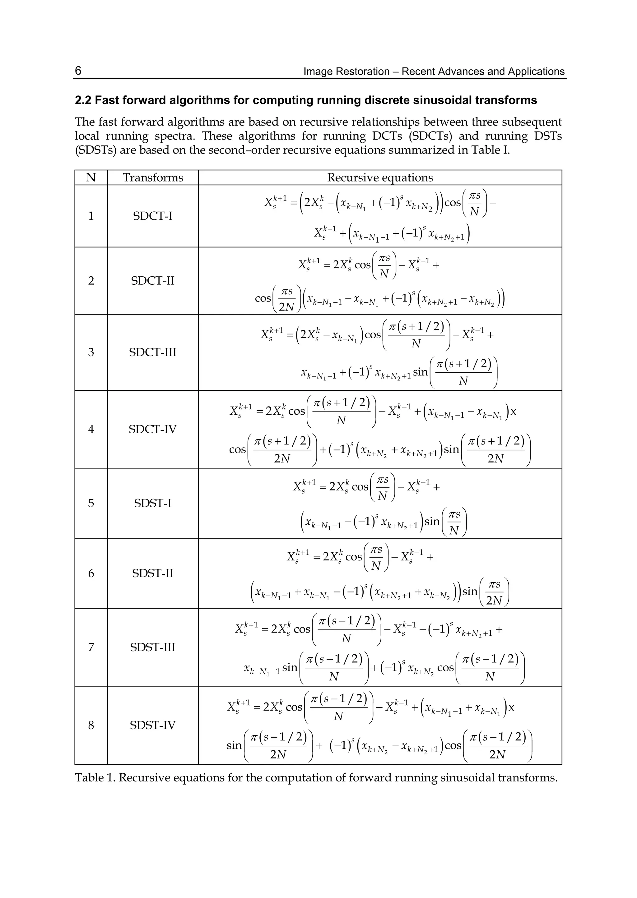
The inverse algorithms for the running DCTs can be written as follows.
IDCT-I:
1
1
1
0
1
1
2 cos 1
N
Nk k k
k s N
s
N s
x X X X
N N
, (11)
where N=N1+N2. If xk is the central pixel of the window; that is, N1=N2 then the inverse
transform is simplified to
1
1
1
2 0
1
1
2 1 1
N
s Nk k k
k s N
s
x X X X
N
. (12)
Therefore, in the computation only the spectral coefficients with even indices are involved.
The number of required operations of multiplication and addition becomes one and N1+1,
respectively.
IDCT-II:
1
1
0
1
1 /21
2 cos
N
k k
k s
s
N s
x X X
N N
, (13)
where N=N1+N2+1. If xk is the central pixel of the window, that is, N1=N2 then the inverse
transform is given by
1
2 0
1
1
2 1
N
s k k
k s
s
x X X
N
. (14)
We see that in the computation only the spectral coefficients with even indices are involved.
The computation requires one multiplication operation and N1+1 addition operations.
IDCT-III:
1
1
0
1 /22
cos
N
k
k s
s
N s
x X
N N
, (15)
where N=N1+N2+1. If xk is the central pixel of the window, that is, N1=N2 then the inverse
transform is
1
1
1 1
1
1
1
[ /2]1
1
0
1 1 1 11 /22
1 cos 1
4
N N
N
N Nk k
k s N s N
s
kN s
x X X X
N N
. (16)
If N1 is even, then the computation requires N1+1 multiplication operations and 2N1
addition operations. Otherwise, the complexity is reduced to N1 multiplication operations
and 2N1 - 1 addition operations.
IDCT-IV:](https://image.slidesharecdn.com/imagerestorationrecentadvancesandapplications-160714160024/75/Image-restoration-recent_advances_and_applications-18-2048.jpg)
![Image Restoration – Recent Advances and Applications10
where N=N1+N2+1. If xk is the central pixel of the window; that is, N1=N2 then we can
rewrite
1
1
1 1
1
1
21
1 1
1
1 1 1 11 1 22
1 sin 1
4
N N
N
N Nk k
k s N s N
s
kN s
x X X X
N N
. (24)
If N1 is even, then the computation requires N1+1 multiplication operations and 2N1
addition operations. Otherwise, the complexity is reduced to N1 multiplication operations
and 2N1 - 1 addition operations.
IDST-IV:
1
1
1 /2 1 /22
sin
N
k
k s
s
N s
x X
N N
, (25)
where =N1+N2+1. If xk is the central pixel of the window; that is, N1=N2, then the inverse
transform is given by
1
11
2 2 1
1
2
1 1
N
s Nk k k
k s s N
s
x X X X
N
. (26)
The complexity is one multiplication operation and N-1 addition operations.
3. Local image restoration with running transforms
First we define a local criterion of the performance of filters for image processing and then
derive optimal local adaptive filters with respect to the criterion. One the most used
criterion in signal processing is the minimum mean-square error (MSE). Since the processing
is carried out in a moving window, then for each position of a moving window an estimate
of the central element of the window is computed. Suppose that the signal to be processed is
approximately stationary within the window. The signal may be distorted by sensor’s noise.
Let us consider a generalized linear filtering of a fragment of the input one-dimensional
signal (for instance for a fixed position of the moving window). Let a=[ak] be undistorted
real signal, x=[xk] be observed signal, k=1,…, N, N be the size of the fragment, U be the
matrix of the discrete sinusoidal transform, E{.} be the expected value, superscript T denotes
the transpose. Let a Hx be a linear estimate of the undistorted signal, which minimizes
the MSE averaged over the window
a a a a
T
MMSE E N . (27)
The optimal filter for this problem is the Wiener filter (Jain, 1989):
1
H ax xxT T
E E
. (28)
Let us consider the known model of a linear degradation:](https://image.slidesharecdn.com/imagerestorationrecentadvancesandapplications-160714160024/75/Image-restoration-recent_advances_and_applications-20-2048.jpg)
![Space-Variant Image Restoration with Running Sinusoidal Transforms 11
,k k n n k
n
x w a v , (29)
where W=[wk,n] is a distortion matrix, ν=[vk] is additive noise with zero mean, k,n=1,…N, N
is the size of fragment. The equation can be rewritten as
x=Wa+v , (30)
and the optimal filter is given by
1
H K W WK W KT T
aa aa
, (31)
where K aa , K , a 0T T T
aa E E E νν ν are the covariance matrices. It is assumed
that the input signal and noise are uncorrelated.
The obtained optimal filter is based on an assumption that an input signal within the
window is stationary. The result of filtering is the restored window signal. This corresponds
to signal processing in nonoverlapping fragments. The computational complexity of the
processing is O(N2). However, if the matrix of the optimal filter is diagonal, the complexity
is reduced to O(N). Such filter is referred as a scalar filter. Actually, any linear filtering can
be performed with a scalar filter using corresponding unitary transforms. Now suppose that
the signal is processed in a moving window in the domain of a running discrete sinusoidal
transform. For each position of the window an estimate of the central pixel should be
computed. Using the equations for inverse sinusoidal transforms presented in the previous
section, the point-wise MSE (PMSE) for reconstruction of the central element of the window
can be written as follows:
2
2
1
N
l
PMSE k E a k a k E l A l A l
, (32)
where A A l H l X l is a vector of signal estimate in the domain of a sinusoidal
transform, HU H l is a diagonal matrix of the scalar filter, l α is a diagonal
matrix of the size xN N of the coefficients of an inverse sinusoidal transform (see Eqs. (12),
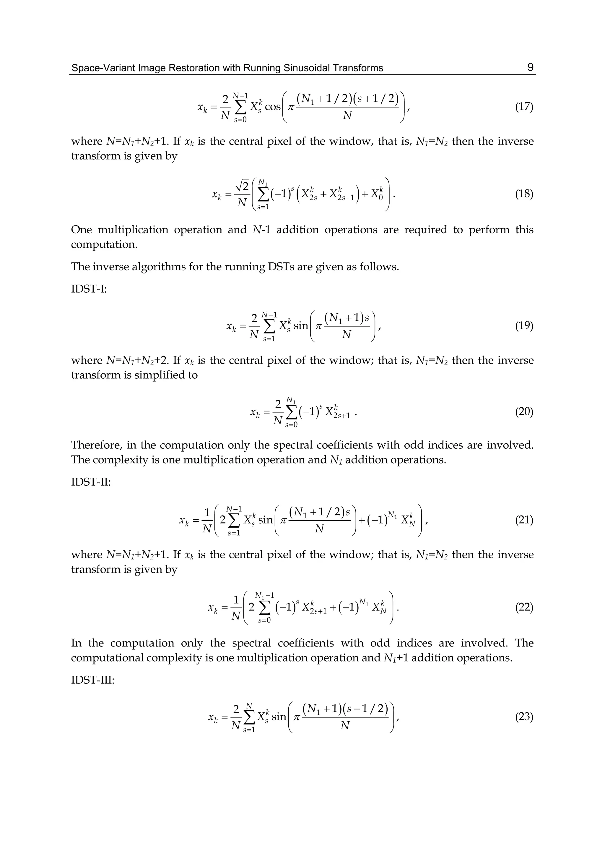
(14), (16), (18), (20), (22), (24), and (26)). Minimizing Eq. (32), we obtain
1
x axH P P IU x
, (33)
where I 1 , 2 ,...,diag N is a diagonal matrix of the size xN N ,
1 if 0, else 0x x , ax xP , PxE A l X k E X l X k . Note that matrix
l α is sparse; the number of its non-zero entries is approximately twice less than the
size of the window signal. Therefore, the computational complexity of the scalar filters in
Eq. (33) and signal processing can be significantly reduced comparing to the complexity for
the filter in Eq. (31). For the model of signal distortion in Eq. (30) the filter matrix is given as](https://image.slidesharecdn.com/imagerestorationrecentadvancesandapplications-160714160024/75/Image-restoration-recent_advances_and_applications-21-2048.jpg)
![Space-Variant Image Restoration with Running Sinusoidal Transforms 15
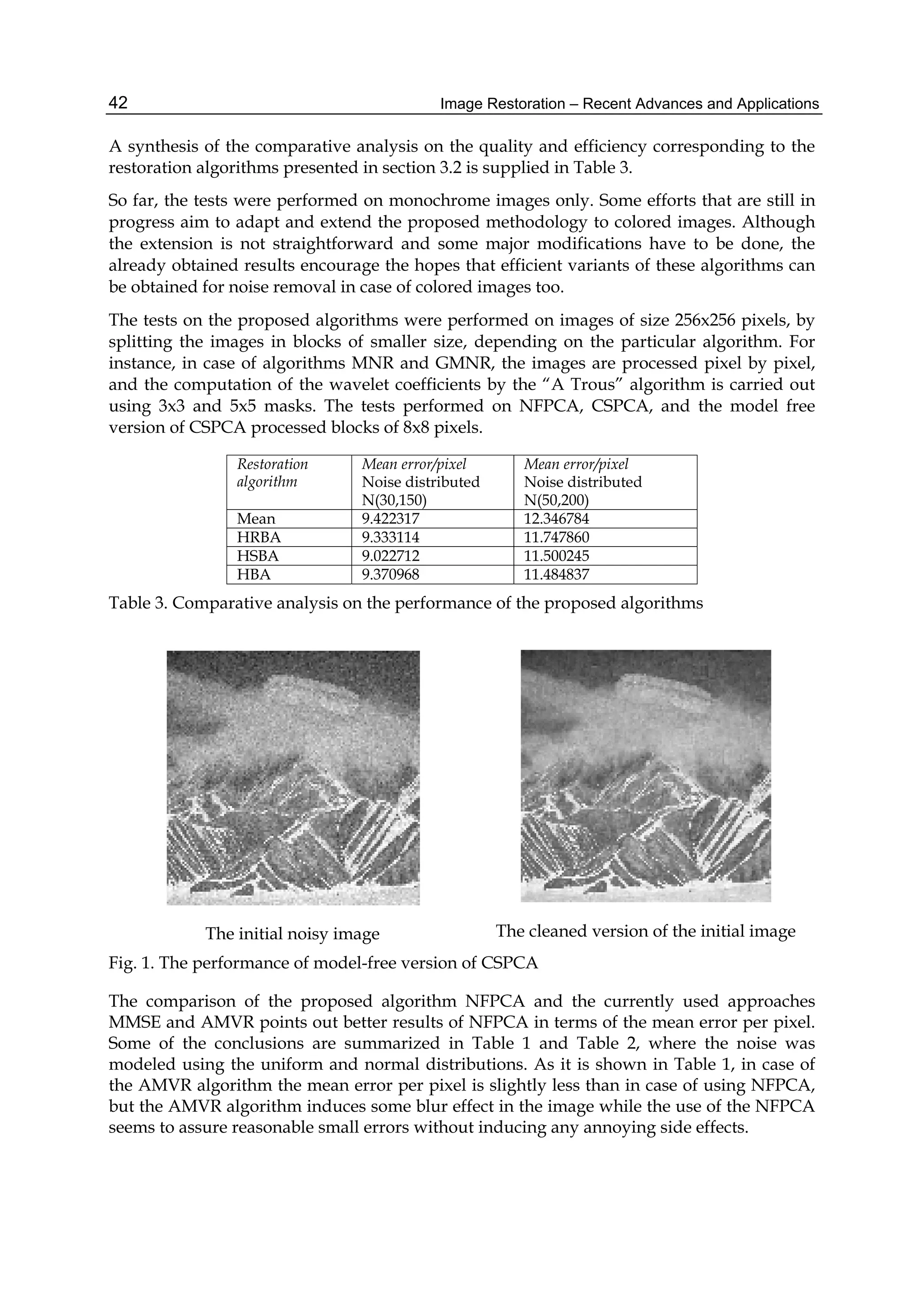
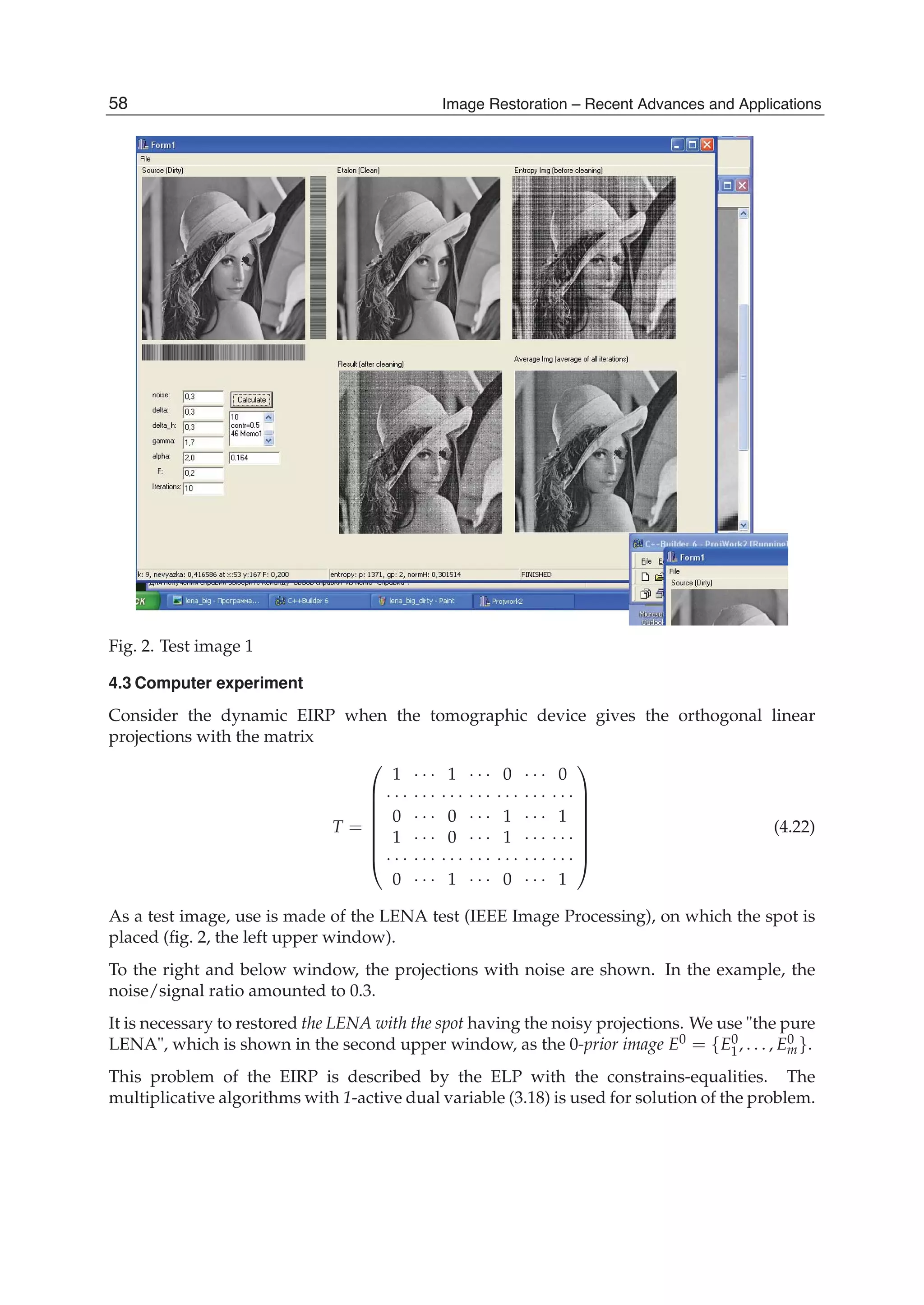
4.2 Local adaptive restoration of real degraded image
A real test aerial image is shown in Fig. 2(a). The size of image is 512x512, each pixel has 256
levels of quantization. The signal range is [0, 1]. The image quadrants are degraded by
running 1D horizontal averaging with the following sizes of the moving window: 5, 6, 4,
and 3 pixels (for quadrants from left to right, from top to bottom). The image is also
corrupted by a zero-mean additive white Gaussian noise. The degraded image with the
noise standard deviation of 0.05 is shown in Fig. 2(b).
In our tests the window length of 15x15 pixels is used, it is determined by the minimal size
of details to be preserved after filtering. Since there exists difference in spectral distributions
of the image signal and wide-band noise, the power spectrum of noise can be easily
measured from the experimental covariance matrix. We carried out three parallel processing
of the degraded image with the use of SDCT-II, SDST-I, and SDST-II transforms. At each
position of the moving window the local correlation coefficient is estimated from the
restored images. On the base of the correlation value and the standard deviation of noise,
the resultant image is formed from the outputs obtained with either SDCT-II or SDST-I, or
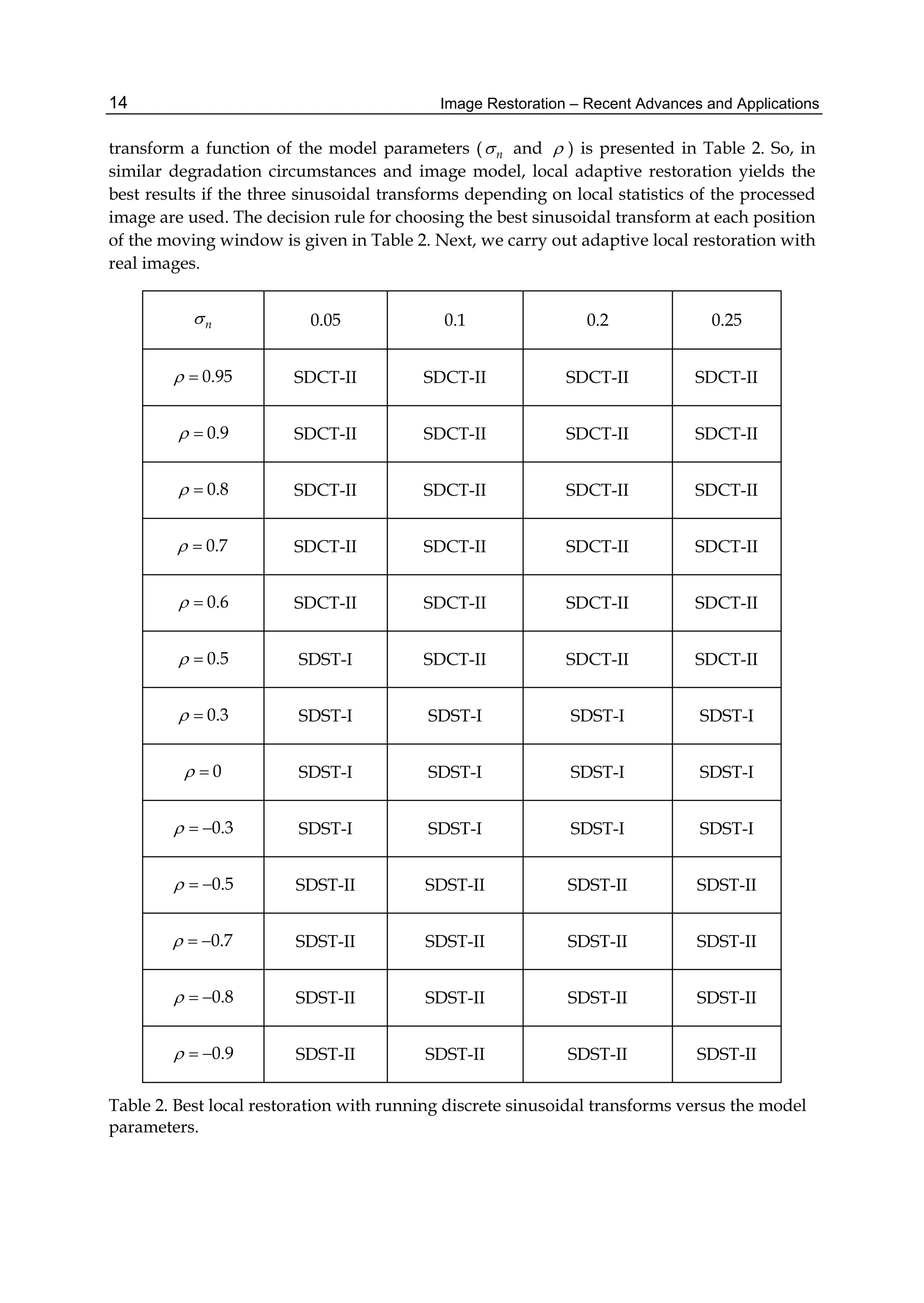
SDST-II according to Table 2.
(a) (b)
Fig. 2. (a) Test image, (b) space-variant degraded test image.
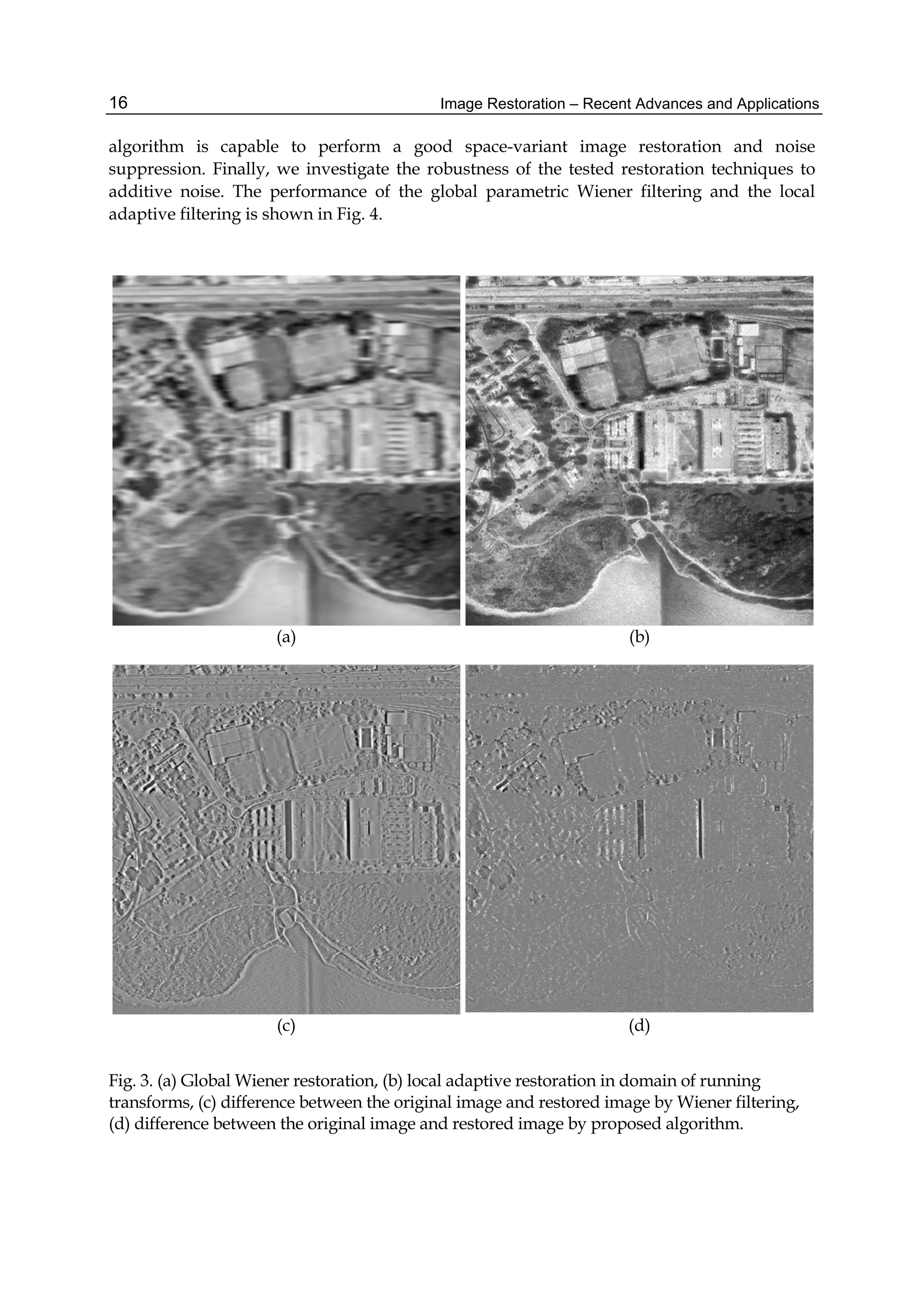
The results of image restoration by the global parametric Wiener filtering (Jain, 1989) and
the proposed method are shown in Figs. 3(a) and 3(b), respectively. Figs. 3(c) and 3(d) show
differences between the original image and images restored by global Wiener algorithm and
by the proposed algorithm, respectively.
We also performed local image restoration using only the SDCT. As expected, the result of
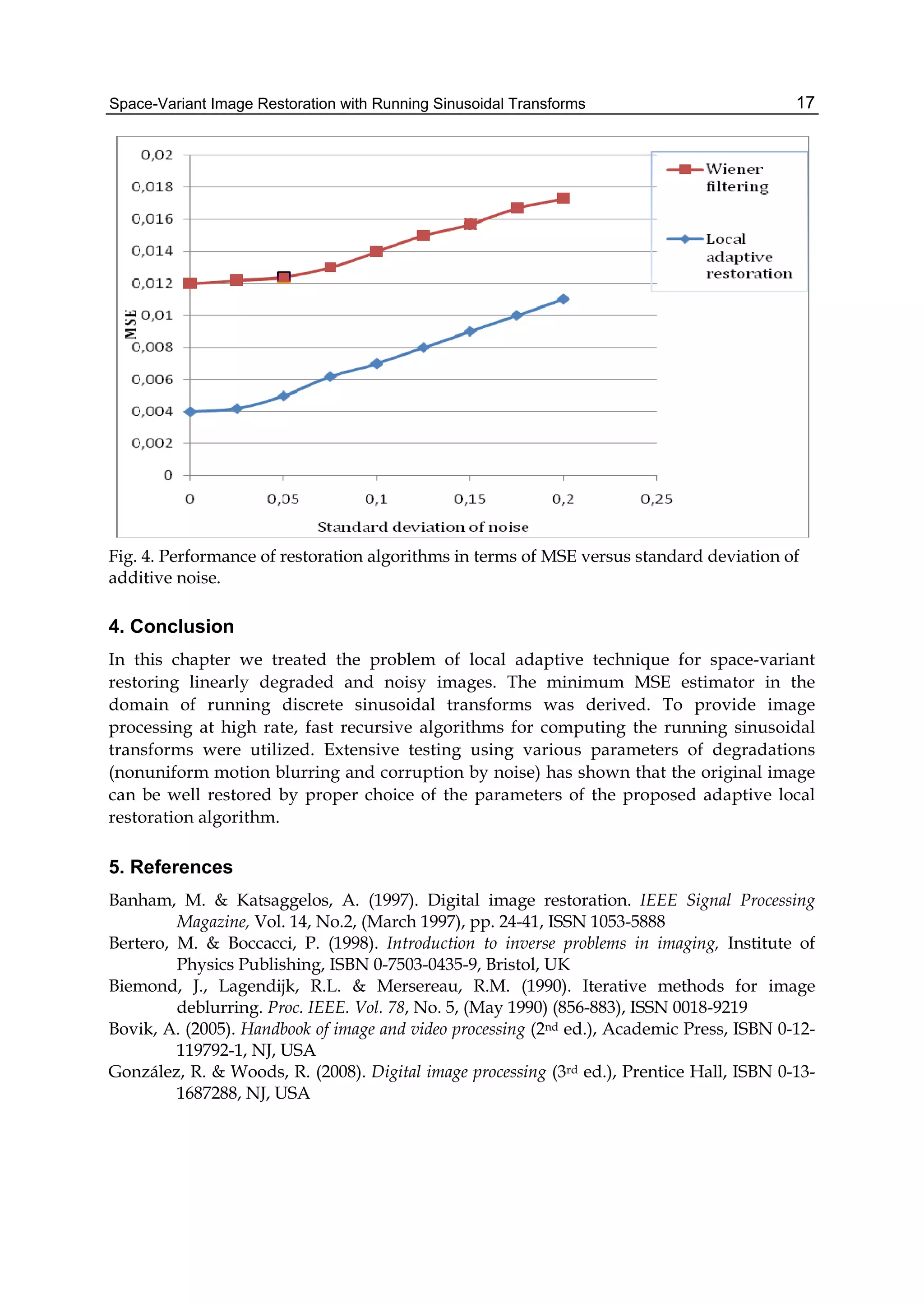
restoration is slightly worse than that of adaptive local restoration. We see that the proposed](https://image.slidesharecdn.com/imagerestorationrecentadvancesandapplications-160714160024/75/Image-restoration-recent_advances_and_applications-25-2048.jpg)

![Statistical-Based Approaches for Noise Removal 25
shows the scatter of samples around their class expected vectors and it is typically given by
the expression
1 1
ˆ ˆ
m N T
i i
w i k i k i
i k
S X X
, where ˆi is the prototype of iH and i is
the a priori probability of , 1,iH i m .
Very often, the a priori probabilities are taken
1
i
m
and each prototype is computed as the
weighted mean of the patterns belonging to the respective class.
The between-class scatter matrix is the scatter of the expected vectors around the mixture
mean as 0 0
1 1
ˆ ˆ
m N
T
b i i i
i k
S
where 0 represents the expected vector of the
mixture distribution; usually 0 is taken as 0
1
ˆ
m
i i
i
.
The mixture scatter matrix is the covariance matrix of all samples regardless of their class
assignments and it is defined by m w bS S S . Note that all these scatter matrices are
invariant under coordinate shifts.
In order to formulate criteria for class separability, these matrices should be converted into a
number. This number should be larger when the between-class scatter is larger or the
within-class scatter is smaller. Typical criteria are 1
1 2 1J tr S S
, 1
2 2 1lnJ S S
, where
1 2, , , , , , , ,b w b m w m m wS S S S S S S S S S and their values can be taken as measures of
overall class separability. Obviously, both criteria are invariant under linear non-singular
transforms and they are currently used for feature extraction purposes [8]. When the linear
feature extraction problem is solved on the base of either 1J or 2J , their values are taken as
numerical indicators of the loss of information implied by the reduction of dimensionality
and implicitly deteriorating class separability. Consequently, the best linear feature
extraction is formulated as the optimization problem *
arg inf ,n m k k
A R
J m A J
where m
stands for the desired number of features , ,kJ m A is the value of the criterion , 1,2kJ k in
the transformed m-dimensional space of T
Y A X , where A is a *n m matrix .
If the pattern classes are represented by the noisy image
X
and the filtered image
F X
respectively, the value of each of the criteria , 1,2kJ k is a measure of overall class
separability as well as well as a measure of the amount of information discriminating
between these classes. In other words, , 1,2kJ k can be taken as measuring the effects of the
noise removing filter expressing a measure of the quantity of information lost due to the use
of the particular filter.
Lemma 3. For any m, 1 m n ,
*
*
1 2arg inf , , ,..., , , 0n m
m m
k k m
A R
J m A J A A R
, where 1 ,..., m are
unit eigenvectors corresponding to the m largest eigenvalues of 1
2 1S S
(Cocianu, State &
Vlamos, 2004).
The probability of error is the most effective measure of a classification decision rule
usefulness, but its evaluation involves integrations on complicated regions in high](https://image.slidesharecdn.com/imagerestorationrecentadvancesandapplications-160714160024/75/Image-restoration-recent_advances_and_applications-35-2048.jpg)
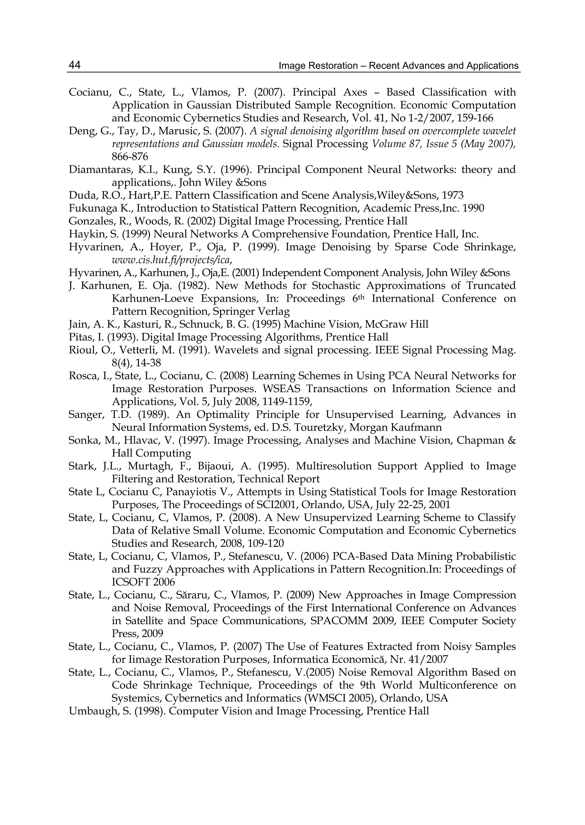
![Statistical-Based Approaches for Noise Removal 41
in Table 1, and Table 2. The aims of the comparative analysis were to establish quantitative
indicators to express both the quality and efficiency of each algorithm. The values of the
variances in modeling the noise in images processed by the NFPCA represent the maximum
of the variances per pixel resulted from the decorrelation process. We denote by U(a,b) the
uniform distribution on the interval [a,b] and by 2
,N the Gaussian distribution of
mean and variance 2
.
It seems that the AMVR algorithm proves better performances from the point of view of mean
error per pixel in case of uniform distributed noise as well as in case of Gaussian type noise.
Also, it seems that at least for 0-mean Gaussian distributed noise, the mask 2h provides less
mean error per pixel when the restoration is performed by the MNR algorithm.
Several tests were performed to investigate the potential of the proposed CSPCA. The tests
were performed on data represented by linearized monochrome images decomposed in
blocks of size 8x8. The preprocessing step was included in order to get normalized, centered
representations. Most of the tests were performed on samples of volume 20, the images of
each sample sharing the same statistical properties. The proposed method proved good
performance for cleaning noisy images keeping the computational complexity at a
reasonable level. An example of noisy image and its cleaned version respectively are
presented in Figure 1.
Restoration algorithm Type of noise Mean error/pixel
MMSE
U(30,80)
52.08
AMVR 10.94
MMSE
U(40,70)
50.58
AMVR 8,07
MMSE
N(40,200)
37.51
AMVR 11.54
GMNR 14.65
NFPCA 12.65
MMSE
N(50,100)
46.58
AMVR 9.39
GMNR 12.23
NFPCA 10.67
Table 1. Comparative analysis on the performance of the proposed algorithms
Restoration algorithm Type of noise Mean error/pixel
MNR
1h
N(0,100)
11.6
MNR
2h 9.53
MNR
1h
N(0,200)
14.16
MNR
2h 11.74
Table 2. Comparative analysis on MNR
The tests performed on new sample of images pointed out good generalization capacities
and robustness of CSPCA. The computational complexity of CSPCA method is less than the
complexity of the ICA code shrinkage method.](https://image.slidesharecdn.com/imagerestorationrecentadvancesandapplications-160714160024/75/Image-restoration-recent_advances_and_applications-51-2048.jpg)
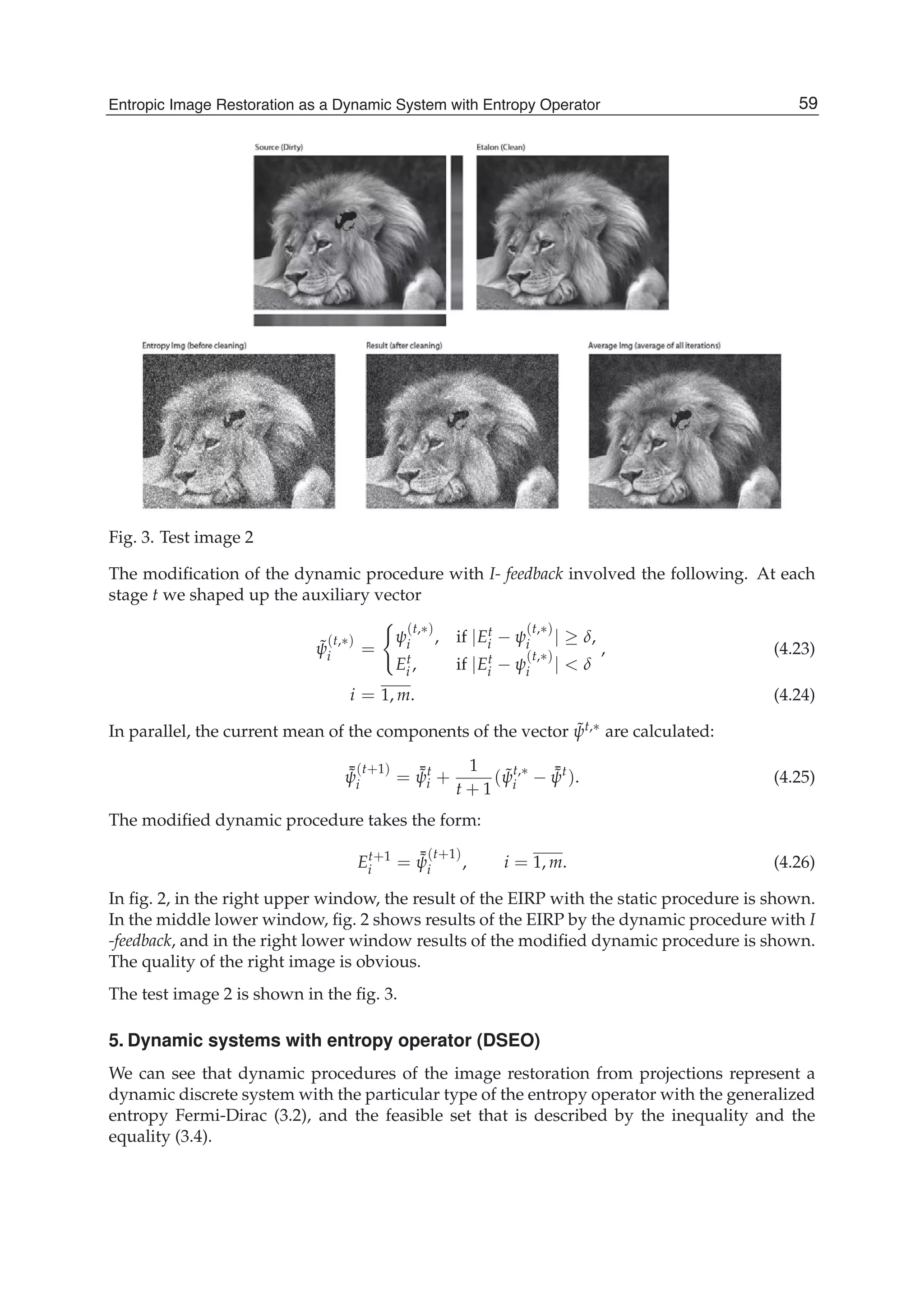
![Entropic Image Restoration as a Dynamic System with Entropy Operator 3
On the each step t of the dynamic procedure t-posterior image is build up as a solution of the
ELP or EQP, using the current t-prior image and the current projection. The (t − s), (t − s +
1), . . . , t-posterior images take part in formation of (t+1)-prior image. So the dynamic procedures
are procedures with feedback.
The dynamic procedures are closed in the sense that at each stage for the current t-prior image
and the t-projection, the entropy-optimal t-posterior image is built up, by which the (t+1)-prior
image is corrected.
We consider a diverse structures of the dynamic procedures with feedback and investigate
their properties. The example of application of these procedures is presented.
It is shown that the proposed dynamic procedures of the EIRP represent the dynamic systems
with entropy operator (DSEO). And our third contribution is an elements of the qualitative
analysis of the DSEO. We consider the properties of the entropy operator (boundedness,
Lipschitz constant).
2. Mathematical model of the static EIRP procedure
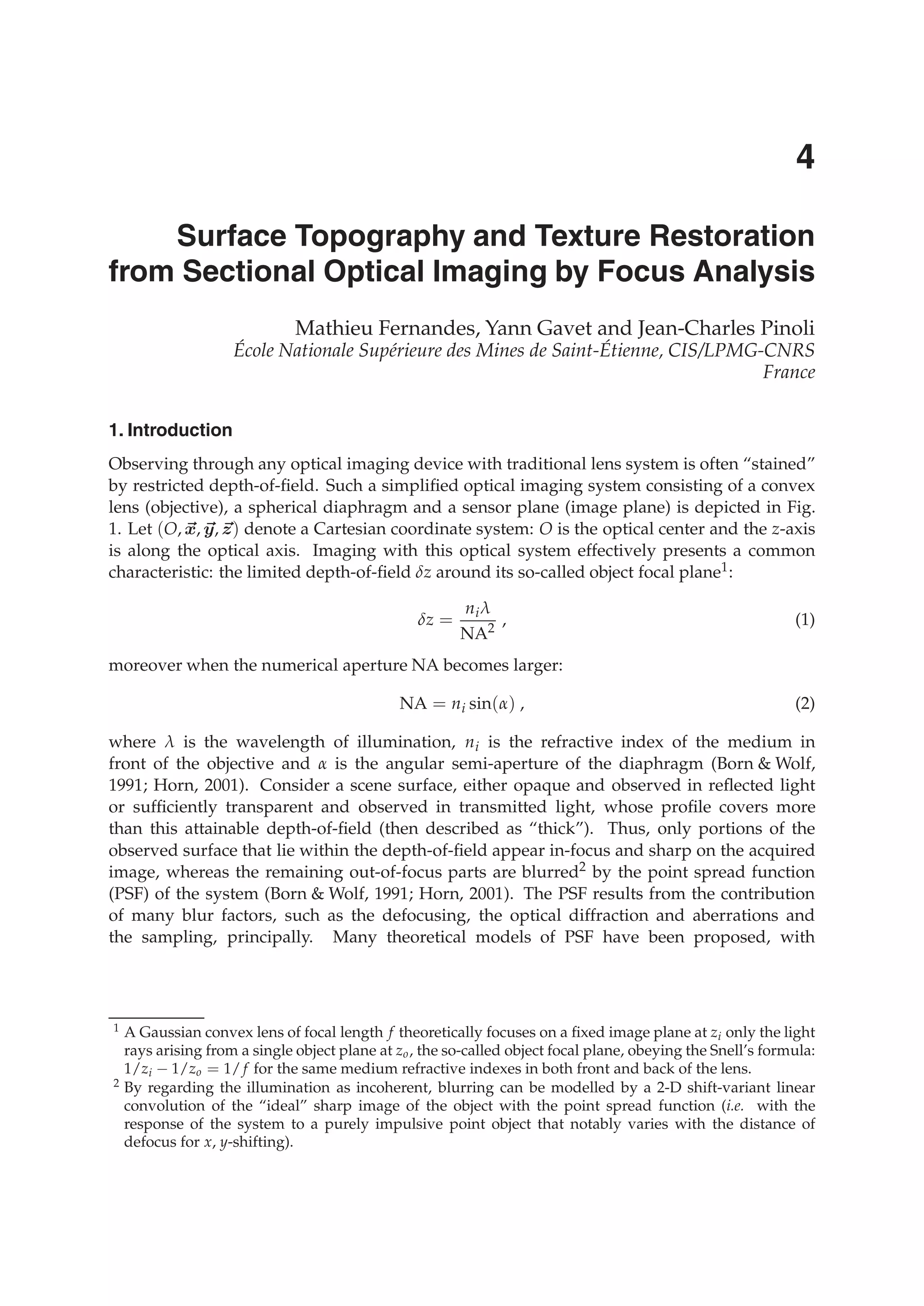
Consider a common diagram of monochrome tomographic investigation (fig. 1), where
external beams of photons S irradiate the flat object in the direction AB. The object is
monochromatic, and is described by the two-dimensional function of optical density ψ(x, y)
in the system of Cartesian coordinates. Positive values of the density function are limited:
0 < a ≤ ψ(x, y) ≤ b < 1. (2.1)
The intensity of irradiation (projection) w at the point B of the detector D (fig. 1) is related by
the Radon transformation:
w(B) = exp −
l∈AB
ψ(x, y)dl , (2.2)
where the integration is realized along straight AB.
It is common to manipulate the digital representation of the density function ψ(l, s), (l =
1, L, s = 1, S). Introduce i = S(l − 1) + s, i = 1, m, m = LS, and martix Ψ = [ψ(l, s)| l =
1, L, s = 1, S] as a vector ¯ψ = {ψ1, . . . , ψm}.
The tomographic procedure form some feasible sets for the vector ¯ψ:
L = { ¯ψ : L( ¯ψ) ≤ g}, (2.3)
where L( ¯ψ) is the h-vector function, and g is the h-vector. We consider the quadratic
approximation of the function L:
L( ¯ψ) = L ¯ψ + Q( ¯ψ), (2.4)
where L is the (h × m)-matrix with nonnegative elements lki ≥ 0; Q( ¯ψ) is the h-vector of the
quadratic forms:
Q( ¯ψ) = ¯ψ Qk ¯ψ, (2.5)
where Qk is the symmetric (m × m)-matrix with elements qk
ij ≥ 0.
47Entropic Image Restoration as a Dynamic System with Entropy Operator](https://image.slidesharecdn.com/imagerestorationrecentadvancesandapplications-160714160024/75/Image-restoration-recent_advances_and_applications-57-2048.jpg)
![4 Will-be-set-by-IN-TECH
Fig. 1. Tomography scheme
Now it is returned to the projection function (2.2), and we use its quadratic approximation:
w(B) T ¯ψ + F( ¯ψ) = u, (2.6)
where: w(B) = {w(B1), . . . , w(Bn)}, T is the (n × m)-matrix with elements tki ≥ 0; F( ¯ψ) is the
n-vector function with components Fr ¯ψ) = ¯ψ Fr ¯ψ, where Fr is the symmetric (m × m)-matrix
with elements fr
ij ≥ 0.
Any tomographic investigation occurs in the presence of noises. So the n-projections vector
u is a random vector with independent components un, n = 1, m, M u = u0 ≥ 0, M (u −
u0)2 = diag [σ2], where u0 is the ideal projections vector (without noise), and σ2 is the
dispersion of the noise. It is assumed that the dispersions of the noise components are equal.
Thus, the feasible set D( ¯ψ) is described the following expressions:
- the projections are
T ¯ψ + F( ¯ψ) = u, (2.7)
- the possible set of the density vectors is
L ¯ψ + Q( ¯ψ) ≤ g. (2.8)
48 Image Restoration – Recent Advances and Applications](https://image.slidesharecdn.com/imagerestorationrecentadvancesandapplications-160714160024/75/Image-restoration-recent_advances_and_applications-58-2048.jpg)
![Entropic Image Restoration as a Dynamic System with Entropy Operator 5
The class P of the density vectors is characterized by the following inequalities:
0 < a ≤ ¯ψ ≤ b < 1. (2.9)
It is assumed that among dimensions of the density vectors (m), the projection vectors (n), and
the possible set (h) the following inequality exists:
m > n + h. (2.10)
It is assumed that the feasible set is nonempty for the class (2.9), and there exists a set of the
density vectors ¯ψ (2.9), that belong to the feasible set D (2.7, 2.8).
We will use the variation principle of the EIRP Popkov (1997), according to which the
realizable density vector (function) ¯ψ maximizes the entropy (the generalized information
entropy by Fermi-Dirac):
H( ¯ψ | a, b, E) = −[ ¯ψ − a] ln
¯ψ − a
E
− [b − ¯ψ] ln[b − ¯ψ], (2.11)
where:
- E = {E1, . . . , Em} is the m-vector characterizing the prior image (prior probabilities of photon
absorption in the object);
- ln[( ¯ψ − a) / E] is the vector with components ln[(ψi − ai) / Ei];
- ln[b − ¯ψ] is the vector with components ln(bi − ψi).
If there is information about more or less "grey" object then we can use the next entropy
function (the generalized information entropy by Boltzmann):
H( ¯ψ | E) = − ¯ψ ln
¯ψ
eE
, (2.12)
where e = 2, 73.
Thus, the problem of the EIRP can be formulated in the next form:
H( ¯ψ | a, b, E) ⇒ max
¯ψ
, ¯ψ ∈ D( ¯ψ) P, (2.13)
where the feasible set D( ¯ψ) is described by the expressions (2.7 - 2.8) and the class P is
described by the inequalities (2.9). This problem is related to the EQP or the ELP depend
on the feasible set construction.
3. Statements and algorithms for the ELP and the EQP
Transform the problem (2.13) to the general form, for that introduce the following
designations:
x = ¯ψ − a, ˜b = b − a,
˜g = g − {a Qk
a, k = 1, h} − La, (3.1)
˜u = u − {a Fr
a, r = 1, n} − Ta.
49Entropic Image Restoration as a Dynamic System with Entropy Operator](https://image.slidesharecdn.com/imagerestorationrecentadvancesandapplications-160714160024/75/Image-restoration-recent_advances_and_applications-59-2048.jpg)
![6 Will-be-set-by-IN-TECH
Then the problem (2.13) takes a form:
H(x, ˜b, E) = −x ln
x
E
− [˜b − x] ln[˜b − x] ⇒ max, (3.2)
under the following constraints:
- the projections
˜Tx + {x Fr
x, r = 1, n} = ˜u, (3.3)
- the possible set
˜Lx + {x Qk
x, k = 1, h} ≤ ˜g, (3.4)
where
˜T = T + AF, , AF = 2[ a Fr
, r = 1, n],
˜L = L + AQ, AQ = 2[ a Qk
, k = 1, h] (3.5)
Remark that the constraints (2.9) are absent in the problem (3.2, 3.4), as they are included to
the goal function.
3.1 The ELP problem
1. Optimality conditions. The feasible set in the ELP problem is described by the next
expressions:
Tx = ˆu, Lx ≤ ˆg, (3.6)
where
ˆu = u − Ta, ˆg = g − La. (3.7)
Consider the Lagrange function for the ELP (3.2, 3.6):
L(x, ¯λ, ¯μ) = H(x, ˜b, E) + [ˆu − Tx] ¯λ + [ˆg − Lx] ¯μ, (3.8)
where ¯λ, ¯μ are the Lagrange multipliers for constraints-equalities and -inequalities (3.6)
correspondingly. Assume that the Slater conditions are valid, i.e., there exists a vector x0
such that Lx0 < ˆg, Tx0 = ˆu.
According to Polyak (1987) the following expressions give the necessary and sufficient
conditions optimality of the triple (x, ¯λ, ¯μ) for the problem (3.2 - 3.5):
∇xL = 0, ∇¯λL = 0, ∇ ¯μL ≥ 0, (3.9)
¯μ ⊗ ∇μL = 0, ¯μ ≥ 0, (3.10)
where ⊗ designates a coordinate-wise multiplication.
The following designations are used in these expressions:
∇xL =
∂H
∂x
− T ¯λ − L ¯μ, (3.11)
∇¯λL = ˆu − Tx, (3.12)
∇ ¯μL = ˆg − Lx, (3.13)
(3.14)
50 Image Restoration – Recent Advances and Applications](https://image.slidesharecdn.com/imagerestorationrecentadvancesandapplications-160714160024/75/Image-restoration-recent_advances_and_applications-60-2048.jpg)
![8 Will-be-set-by-IN-TECH
The parameters γ, α are the step coefficients. In Popkov (2006) the multiplicative algorithms
in respect to the mixed type (prime and dual variables) are introduced, and the method of the
convergence of these algorithms are proposed.
3.2 The EQL problem
1. Optimality condition. Consider the EQL problem (3.2 - 3.5), and introduce the Lagrange
function:
L(x, ¯λ, ¯μ) = H(x, ˜b, E) + ¯λ [ ˜u − ˜Tx − {x Fr
x, r = 1, n}] + (3.20)
+ ¯μ [ ˜g − ˜Lx − {x Qk
x, k = 1, h} ].
According to the optimality conditions (3.9, 3.10) we have:
∇xL =
∂H
∂x
− [ T + Φ(x) ] ¯λ − [ L + Π(x) ] ¯μ = 0,
∇¯λL = ˜u − Tx − {x Fr
x, r = 1, n}, (3.21)
∇ ¯μL = ˜g − Lx − {x Qk
x, k = 1, n} ≥ 0,
¯μ ⊗ ∇ ¯μL = 0, x ≥ 0, ¯μ ≥ 0,
where
Φ(x) = [ϕri(x) | r = 1, n, i = 1, m], ϕri(x) = 2
m
∑
j=1
xj fr
ij,
Π(x) = [πki(x) | k = 1, h, i = 1, m], πkj(x) = 2
m
∑
j=1
xjqk
ij.
Transform these equations and inequalities to the conventional form in which all variables are
nonnegative one:
Aj(x, z, ¯μ) Ej
xj[1 + Aj(x, z, ¯μ) Ej]
= Aj(x, z, ¯μ) = 1, j = 1, m,
1
˜ur
m
∑
i=1
˜trixi +
m
∑
i,l=1
xi xl fr
il = Br(x) = 1, r = 1, n, (3.22)
μk
˜gk
m
∑
i=1
˜lkixi +
m
∑
i,l=1
xi xl qk
il = Ck(x) = 0, k = 1, h,
x ≥ 0, z = exp(−¯λ) ≥ 0, ¯μ ≥ 0,
where
Aj(x, z, ¯μ) =
n
∏
r=1
z
˜trj
r
n
∏
p=1
z
ϕrj(x)
r ×
× exp −
h
∑
k=1
μk
˜lkj exp −
h
∑
k=1
μk
m
∑
l=1
xlqk
jl . (3.23)
52 Image Restoration – Recent Advances and Applications](https://image.slidesharecdn.com/imagerestorationrecentadvancesandapplications-160714160024/75/Image-restoration-recent_advances_and_applications-62-2048.jpg)
![Entropic Image Restoration as a Dynamic System with Entropy Operator 9
2. Multiplicative algorithms of the mixed type with (p+q+w)-active variables. We use p
active prime x variables, q active dual variables z for the constraints-equalities, and w active
dual ¯μ variables for the the constraints-inequalities. The algorithm takes a form:
(a)initial step
x0
≥ 0, z0
≥ 0, ¯μ0
≥ 0;
(b)iterative step
xs+1
j1(s)
= xs
j1(s)A
β
j1(s)
(xs
, zs
, ¯μs
),
· · · · · · · · · · · · , (3.24)
xs+1
jp(s)
= xs
jp(s)A
β
jp(s)
(xs
, zs
, ¯μs
),
xs+1
j = xs
j , j = 1, m, j = j1(s), . . . , jp(s);
zs+1
t1(s)
= zs
t1(s)Bγ
t1
(xs
),
· · · · · · · · · · · · , (3.25)
zs+1
tq(s)
= zs
tq(s)Bγ
tq
(x)s
,
zs+1
t = zs
t, t = 1, n, t = t1(s), . . . , tq(s);
μs+1
k1(s)
= μs
k1(s)[1 − αCk1
(xs
)],
· · · · · · · · · · · · , (3.26)
μs+1
kw(s)
= μs
kw(s)[1 − αCkw
(xs
)],
μs+1
k = μs
k, k = 1, h, k = k1(s), . . . , kw(s);
The parameters β, γ, α are the step coefficients.
3. Active variables. To choice active variables we use feedback control with respect to the
residuals on the each step of iteration. Consider the choosing rule of the active variables for
the ELP problem (3.2, 3.3, 3.4). Introduce the residuals
ϑi(zs
, ¯μs
) = |1 − Θi(zs
, ¯μs
)|, i = 1, n;
εk(zs
, ¯μs
) = μkΓk(zs
, ¯μs
), k = 1, h. (3.27)
One of the possible rules is a choice with respect the maximum residual. In this case it is
necessary to select p maximum residual ϑi1
, . . . , ϑip
and q maximum residual εk1
, . . . , εkq
for
the each iterative step s. The numbers i1, . . . , ip and k1, . . . , kq belong to the intervals [1, n] and
[1, h] respectively.
Consider the step s and find the maximal residual ϑi1
(zs, ¯μs) among ϑ1(zs, ¯μs), . . . , ϑn(zs, ¯μs).
Exclude the residual ϑi1
(zs, ¯μs) from the set ϑ1(zs, ¯μs),
. . . , ϑn(zs, ¯μs), and find the maximal residual ϑi2
(zs, ¯μs) among ϑ1(zs, ¯μs), . . . ,
ϑi1−1(zs, ¯μs), ϑi1+1(zs, ¯μs)ϑn(zs, ¯μs), and etc., until all p maximal residuals will be found.
Selection of the maximal residuals εk1
(zs, ¯μs), . . . , εkq
(zs, ¯μs) is implemented similary.
53Entropic Image Restoration as a Dynamic System with Entropy Operator](https://image.slidesharecdn.com/imagerestorationrecentadvancesandapplications-160714160024/75/Image-restoration-recent_advances_and_applications-63-2048.jpg)
![10 Will-be-set-by-IN-TECH
Now we represent the formalized procedure of selection. Introduce the following
designations:
n
p
= I + δ, I =
n
p
, 0 ≤ δ ≤ p − 1;
h
q
= J + ω, J =
h
q
, 0 ≤ ω ≤ q − 1. (3.28)
= s (mod (I + 1)), κ = s (mod (J + 1)). (3.29)
Consider the index sets:
N = {1, . . . , n} Nr(s) = {i1(s), . . . , ir(s)};
K = {1, . . . , h} Kv(s) = {k1(s), . . . , kv(s)}, (3.30)
where
r =
⎧
⎪⎪⎪⎨
⎪⎪⎪⎩
[1, p], if < I;
[1, δ], if = I;
0, if δ = 0
, v =
⎧
⎪⎪⎪⎨
⎪⎪⎪⎩
[1, q], if κ < J;
[1, ω] if κ = J;
0, if ω = 0.
(3.31)
Introduce the following sets:
Pr−1(s) =
l=1
Np(s − l) Nr−1(s), Gr−1 = N Pr−1(s).
Qv−1(s) =
κ
l=1
Kv(s − l) Kv−1(s), Rv−1 = K Qv−1(s).
(3.32)
The numbers r and v are determined by the equalities (3.31), and
N0(s) = K0(s) = P0(s) = G0(s) = Q0(s) = R0(s) = ∅, for all s.
Now we define the rule of the (p+q)-maximal residual in the following form:
ij(s) = arg max
[i∈Gj−1(s)]
ϑi(zs
, ¯μs
),
kl(s) = arg max
[k∈Rl−1(s)]
εk(zs
, ¯μs
). (3.33)
According to this rule we have the chain of inequalities:
ϑip
(zs
, ¯μs
) < ϑip−1
(zs
, ¯μs
) < · · · < ϑi1
(zs
, ¯μs
),
εkq
(zs
, ¯μs
) < εkq−1
(zs
, ¯μs
) < · · · < εk1
(zs
, ¯μs
). (3.34)
We can see that all dual variables are sequentially transformed to active ones during I + J + 2
iterations It is repeated with a period of I + J + 2.
54 Image Restoration – Recent Advances and Applications](https://image.slidesharecdn.com/imagerestorationrecentadvancesandapplications-160714160024/75/Image-restoration-recent_advances_and_applications-64-2048.jpg)
![12 Will-be-set-by-IN-TECH
In the second case, information collections at t, t − 1, . . . , t − s stages are used for the estimation
of the current mean ¯¯ψt of the posterior image:
E(t+1)
= L(Et
, ¯¯ψt
). (4.7)
Finally, in the third case, information collections at t, t − 1, . . . , t − s stages are used for the
estimation of the current mean ¯¯ψt and dispersion dt
of the posterior image:
E(t+1)
= L(Et
, ¯¯ψt
, dt
). (4.8)
We will introduce the following types of the dynamic procedures of the EIRP:
• the identical feedback (I − f eedback)
E(t+1)
= arg max
ψt
H( ¯ψt
)|Et
) | ¯ψt
∈ D(ut
); (4.9)
• the feedback with respect to the current mean of image (CM − f eedback)
E(t+1)
= Et
+ α(Et
− ¯¯ψt
), (4.10)
¯¯ψ(t+1)
= ¯¯ψt
+
1
t + 1
ψ(t,∗)
− ¯¯ψt
;
¯ψ(t,∗)
= arg max
ψ
{H( ¯ψt
, Et
)| ¯ψt
∈ D(ut
)};
(4.11)
• the feedback with respect to the current mean and dispersion of image (CMD − f eedback)
E(t+1)
= Et
+ α(dt
)(Et
− ¯¯ψt
), (4.12)
¯¯ψ(t+1)
= ¯¯ψt
+
1
t + 1
¯ψ(t,∗)
− ¯¯ψt
, (4.13)
d(t+1)
= dt
+
1
t + 1
dt
+ [ ¯ψ(t,∗)
− ¯¯ψt
]2
,
¯ψ(t,∗)
= arg max
ψ
{H( ¯ψ, Et
) | ¯ψt
∈ D(ut
)}.
(4.14)
4.2 Investigation of the dynamic EIRP procedure with I-feedback
Consider the problem (2.13) in which the feasible set is the polyhedron, a = 0, b = 1, and the
constraints to the possible density functions (2.7) are absent. In this case t-posterior density
function hold:
ψt,∗
i =
Et
i
Et
i + ∏n
j=1[zt
j]tji
, i = 1, m. (4.15)
The exponential Lagrange multipliers z1, . . . , zn are defined from the following equations:
Φj(zt
) =
m
∑
i=1
tjiEt
i
Et
i + ∏n
j=1[zt
j]tji
= uj, j = 1, n. (4.16)
56 Image Restoration – Recent Advances and Applications](https://image.slidesharecdn.com/imagerestorationrecentadvancesandapplications-160714160024/75/Image-restoration-recent_advances_and_applications-66-2048.jpg)
![Entropic Image Restoration as a Dynamic System with Entropy Operator 13
According to the definition of the I-feedback procedure we have:
Et+1
i = Ψi(Et
) =
Et
i
Et
i + ϕi[zt(Et)]
, i = 1, m, (4.17)
where
ϕi[zt
(Et
)] =
n
∏
j=1
[zt
j]tji
≥ 0. (4.18)
The iterative process (4.17) can be considered as the method of the simple iteration applying
to the eguations:
Ei =
Ei
Ei + ϕi[z(E)]
, i = 1, m. (4.19)
Theorem 1.Let ϕi[z(E)] ≤ 1 for all i = 1, m, z ≥ 0, 0 ≤ E ≤ 1.
Then the system of equations (4.19) has the unique solution E∗.
Proof. Consider the auxiliary equation:
x = Ψ(x) =
x
x + a
, x ≥ 0.
We can see that the function Ψ(x) is strictly monotone increasing (Ψ (x) > 0 for all x > 0 and Ψ(∞) = 0),
and is strictly convex (Ψ (x) < 0, x > 0 and Ψ (∞) = 0).
If Ψ (0) = 1/a ≥ 1, (a ≤ 1), then the auxiliary equation has the unique solution, and the method of the
simple iteration is converged to this solution.
Now it is necessary to find a conditions when ϕi[z(E)] ≤ 1. The sufficient conditions for it is
formed by the following theorem.
Theorem 2. Let the matrix T in (2.7) has the complete rank n, and the following conditions be valid:
max
j∈[1,n]
m
∑
i=1
tji − umax > 0, umax = max
j∈[1,n]
uj; (4.20)
min
j∈[1,n]
m
∑
i=1
tji
Et
i
Et
i + 1
− umin < 0, umin = min
j∈[1,n]
uj. (4.21)
Then ϕi[z(E)] ≤ 1 for all i = 1, m.
Proof. Consider the Jacobian of the vector-function ¯Φ(zt). Its elements take a form:
∂Φj(zt)
∂zk
= −
1
zk
m
∑
i=1
tji tki Et
i ϕi(zt)
[Et
i + ϕi(zt)]2
≤ 0, (j, k) = 1, n.
The equality to zero is reached when z → ∞. So, the functions Φ1, . . . , Φn are strictly monotone
decreasing.
Therefore, under the theorem’s conditions, the solution of the equations (4.16) z∗
j ∈ [0, 1], j = 1, n, and
the functions 0 < φj(z(E)) ≤ 1.
57Entropic Image Restoration as a Dynamic System with Entropy Operator](https://image.slidesharecdn.com/imagerestorationrecentadvancesandapplications-160714160024/75/Image-restoration-recent_advances_and_applications-67-2048.jpg)
![16 Will-be-set-by-IN-TECH
In general case the class of the continuous DSEO is described by the following differential
equations:
du(t)
dt
= U (u(t), v(t), y[t, u(t), v(t)]) , u(0) = u0
. (5.1)
dv(t)
dt
= V (u(t), v(t), y[t, u(t), v(t)]) , v(0) = v0
. (5.2)
with the entropy operator:
y[t, u(t), v(t)] = arg max
y
{H(t, y, u(t)) | y ∈ D[t, v(t)]} , (5.3)
where: H(t, y | u) is an entropy function with the H-parameters u; the vectors (y, u) ∈
Rn, v ∈ Rm , and D(t, v) is a feasible set depended from the D-parameters v.
In these equations U is the n-vector-function, and V is the m-vector-function.
5.1 Classification of the DSEO
Some physical analogues we will use for construction of the classificatory graph. In particular,
from the equations (5.1, 5.2) it is seen the rates of parameters is proportional to the flows. The
entropy function is a probability characteristics of a stochastic process. So the H-parameters
are the parameters of this process.
We will use the following classificatory indicators:
• (A), types of the state coordinates ( H -coordinates u, D -coordinates v,
HD -coordinates u, v);
• (B), flows ( Add - an additive flow, Mlt - a multiplicative flow);
• (C), entropy functions ( F -Fermi-, E -Einstein-, B -Boltzmann-entropy functions);
• (D), models of the feasible sets ( Eq -equalities, Ieq -inequalities, Mx -mixed);
• (F), types of the feasible sets ( Plh - polyhedron, Cnv -convex, nCnv -non-convex).
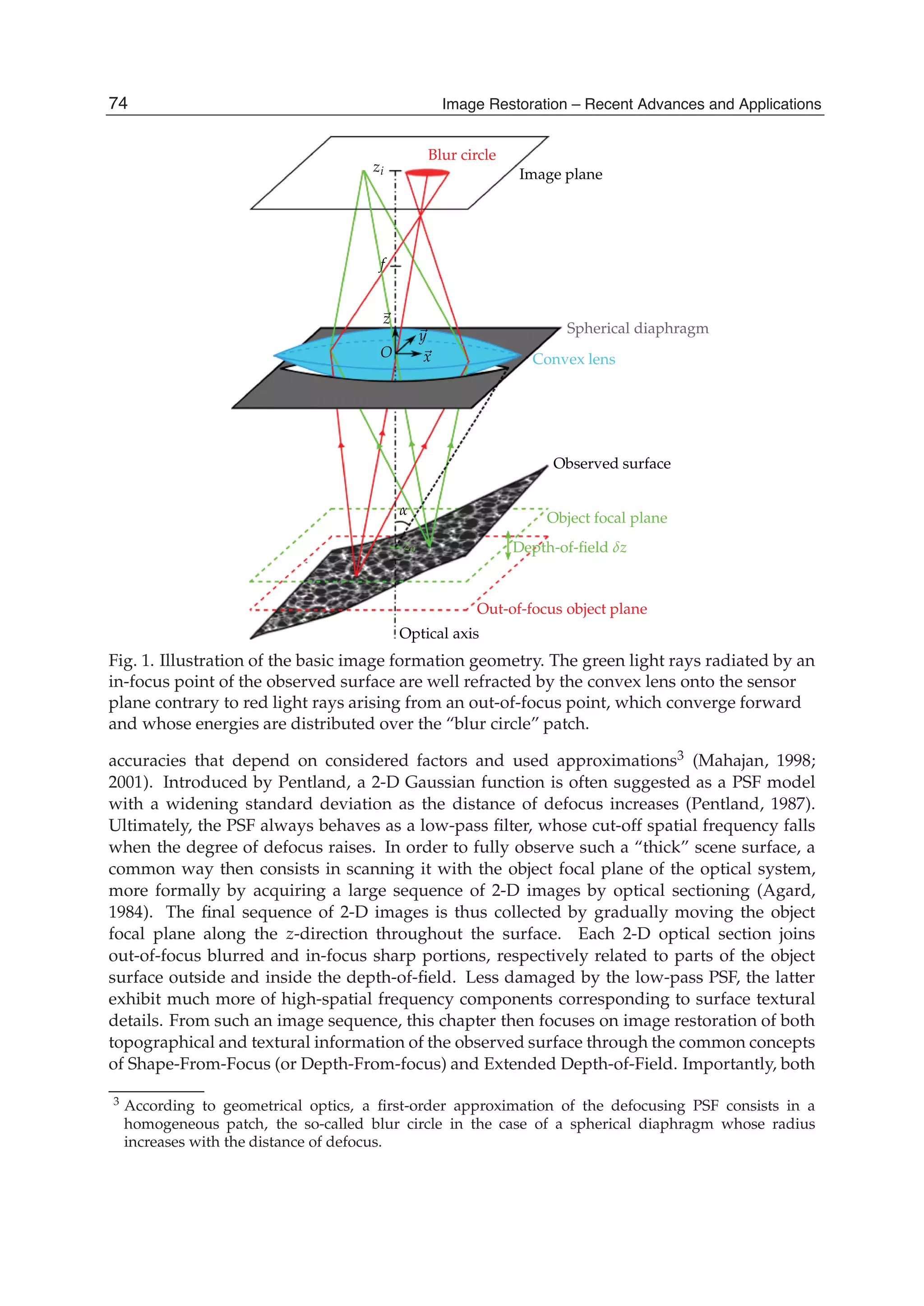
The classificatory graph is shown in the fig. 4.
At the beginning we consider some properties of the entropy operator, notably, the
HD, B, Eq, Plh -entropy operator that is included to the HD -DSEO:
y[u, v] = arg max HB[y, u] | y ∈ ˜D[v] , (5.4)
where Boltzmann-entropy function is
H(y | u) = − y ln
y
eu
, y ∈ Rm
+, (5.5)
and the feasible set is
˜D[v] = {y : ˜T y = v, y ≥ 0}. (5.6)
In these expressions the vector ln
y
eu = {ln
y1
eu1
, . . . , ln
ym
eum
}, and the vectors
u ∈ Um
+(u−
, u+
) ⊂ Rm
+, v ∈ Vn
+(v−
, v+
) ⊂ Rn
+, n < m, (5.7)
and
Um
+(u−
, u+
) = {u : 0 < u−
≤ u ≤ u+
≤ 1},
Vn
+(v−
, v+
) = {v : 0 < v−
≤ v ≤ v+
}. (5.8)
The (n × m)-matrix ˜T = [˜tki ≥ 0] has a full rank equal n.
60 Image Restoration – Recent Advances and Applications](https://image.slidesharecdn.com/imagerestorationrecentadvancesandapplications-160714160024/75/Image-restoration-recent_advances_and_applications-70-2048.jpg)
![Entropic Image Restoration as a Dynamic System with Entropy Operator 17
Fig. 4. Classificatory graph
5.2 Estimation of the local Lipschitz-constants for the HD, B, Eq, Plh -entropy operator.
The HD, B, Eq, Plh -entropy operator describes the mapping of the sets Um
+(u−, u+) and
Vn
+(v−, v+) into the set Y ⊂ Rm
+ of the operator’s values. We will characterize this mapping
by two local Lipschitz-constants - LU and LV, i.e.
y[u(1)
, v(1)
] − y[u(2)
, v(2)
] ≤ LU u(1)
− u(2)
+ LV v(1)
− v(2)
. (5.9)
We will use the upper estimations of local Lipschitz-constant:
LU ≤ max
Um
+
YU , LV = max
Vn
+
YV , (5.10)
where YU and YV are the U-Jacobian and the V-Jacobian of the operator y[u, v] respectively.
Evaluate the normalized entropy operator in the following form:
x(u, v) = arg max (H[x, u] | Tx = v, x ≥ 0) , (5.11)
where
H(x | u) = − x ln
x
eu
. (5.12)
ti =
n
∑
k=1
˜tki, tki =
˜tki
ti
, i = 1, m. (5.13)
The matrix T in (5.11) has a full rank n and the normalized elements, i.e. ∑n
k=1 tki = 1 for
all i = 1, m. Also it is assumed that the condition of the dominating diagonal is valid for the
quadratic matrix T T , i.e. the following inequalities take a form:
m
∑
i=1
⎛
⎝t2
ki −
n
∑
j=k
tkitji
⎞
⎠ ≥ > 0, k = 1, n. (5.14)
61Entropic Image Restoration as a Dynamic System with Entropy Operator](https://image.slidesharecdn.com/imagerestorationrecentadvancesandapplications-160714160024/75/Image-restoration-recent_advances_and_applications-71-2048.jpg)
![18 Will-be-set-by-IN-TECH
The feasible set D = {x : T x = v, x ≥ 0} is not empty, notable, there exists some subset of
the nonnegative vectors x ∈ D.
Designate the Lipschitz-constant for the normalized operator (5.11) as ˜LU and ˜LV respectively,
i.e.
x[u(1)
, v(1)
] − x[u(2)
, v(2)
] ≤ ˜LU u(1)
− u(2)
+ ˜LV v(1)
− v(2)
. (5.15)
We will use the upper estimations of local Lipschitz-constant:
˜LU ≤ max
Um
+
XU , ˜LV = max
Vn
+
XV , (5.16)
where XU and XV are the U-Jacobian and the V-Jacobian of the operator x[u, v] respectively.
According to (5.13), the following relation between the operators y(u, v) (5.4) and x(u, v) (5.11)
exists:
y(u, v) = t−1
⊗ x(u, v), (5.17)
where the vector t−1 = {t−1
1 , . . . , t−1
m }, where the components ti are defined by the equalities
(5.13), and ⊗ implies the coordinate-wise multiplication of the vectors.
Thus we have the following equalities:
LU = t−1 ˜LU, LV = t−1 ˜LV, (5.18)
Thus, we will calculate the local Lipschitz-constants estimations for the normalized entropy
operator (5.11, 5.12) and then apply the formulas (5.17, 5.18).
The normalized entropy operator x(u, v) can be represented by the form:
xi(u, v) = ui exp
⎛
⎝−
n
∑
j=1
λj(u, v) tji
⎞
⎠ , i = 1, m, (5.19)
where the Lagrange multipliers λj(u, v), (j = 1, n) as the implicit functions from u, v define
by the equations:
Φk[u, λ(u, v)] =
m
∑
i=1
uitki exp
⎛
⎝−
n
∑
j=1
λj(u, v) tji
⎞
⎠ = vk, k = 1, n. (5.20)
1. Estimations of the norm’s matrix XU. The (m × m)-matrix XU takes a form:
XU =
∂xi
∂uj
, (i, j) = 1, m ,
We will use Euclidean vector norm ( y 2), with which two matrix norm are consisted (see Voevodin
(1984)):
- the spectral norm
A 2 =
√
σmax,
where σmax is the maximal eigenvalue of the matrix A;
62 Image Restoration – Recent Advances and Applications](https://image.slidesharecdn.com/imagerestorationrecentadvancesandapplications-160714160024/75/Image-restoration-recent_advances_and_applications-72-2048.jpg)
![Entropic Image Restoration as a Dynamic System with Entropy Operator 19
- and the Euclidean norm
A E = ∑
i,j
|aij|2.
It is known that
A 2 ≤ A E
It is assumed that XU = XU 2. We have from (5.19) the following equality:
XU = Xu + Xλ ΛU, (5.21)
where the (m × m)-matrix
Xu = diag [
xi
ui
| i = 1, m]; (5.22)
the (m × n)-matrix
Xλ = −x ⊗ T ; (5.23)
and the n × m-matrix
ΛU =
∂λj
∂ui
, j = 1, n, i = 1, m (5.24)
In these expressions ⊗ is coordinate-wise multiplication of the vector’s components to the
rows of the matrix.
According to (5.21) and the relation between the spectral norm and the Euclidean norm, we
have:
XU 2 ≤ Xu E + Xλ E ΛU E, (5.25)
where
Xu E ≤
√
m
xmax
u−
min
, (5.26)
xmax
= max
(i,u,v)
xi(u, v), u−
min = min
i
u−
i . (5.27)
Xλ E ≤ xmax
T E = xmax
m,n
∑
i=1,j=1
t2
ij. (5.28)
Now consider the equations (5.20), and differentiate the left and right sides of these equations
by u. We obtain the following matrix equation:
Φλ ΛU = −Φu, (5.29)
From this implies that
ΛU =
∂λk
∂ui
| k = 1, n, i = 1, m = −Φ−1
λ Φu. (5.30)
Here the (n × n)-matrix Φλ has elements
φλ
ks = −
m
∑
i=1
uitkitjs exp
⎛
⎝−
n
∑
j=1
λj(u, v)tji
⎞
⎠ , (k, s) = 1, n; (5.31)
63Entropic Image Restoration as a Dynamic System with Entropy Operator](https://image.slidesharecdn.com/imagerestorationrecentadvancesandapplications-160714160024/75/Image-restoration-recent_advances_and_applications-73-2048.jpg)
![Entropic Image Restoration as a Dynamic System with Entropy Operator 21
Thus the norm’s estimation of the matrix XV takes a form:
XV 2 ≤ Φ−1
λ 2 xmax
m,n
∑
i=1,j=1
t2
ij. (5.43)
So, we can see that it is necessary to construct the norm’s estimation for the matrix Φ−1
λ , as
well as for the norm’s estimation of the matrix XU .
3. Estimation of the spectral norm of the matrix Φ−1
λ . The matrix Φλ (5.31) is symmetric and
strictly negative defined for all λ. Therefore, it has n real, various, and negative eigenvalues
(see Wilkinson (1970)). We will order them in the following way:
μ1 = μmin < μ2 < · · · < μn = μmax < 0, |μmax| > M. (5.44)
The spectral norm of an inverse matrix is equal to the inverse value of the modulus of the
maximum eigenvalue μmax of the initial matrix, i.e.
Φ−1
λ ≤ M−1
. (5.45)
To definite the value M we resort to the Gershgorin theorem (see Wilkinson (1970)). According
to the theorem any eigenvalue of a symmetric strictly negative definite matrix lies at least in
one of the intervals with center −ck(λ) and the width 2 ρk(λ):
− g+
k (λ) = −ck(λ) − ρk(λ) ≤ μ ≤ −ck(λ) + ρk(λ) = −g−
k (λ), k = 1, n, (5.46)
where according to (5.19)
g+
k (λ) =
m
∑
i=1
xi
⎛
⎝t2
ki +
n
∑
j=k
tkitji
⎞
⎠ ,
g−
k (λ) =
m
∑
i=1
xi
⎛
⎝t2
ki −
n
∑
j=k
tkitji
⎞
⎠ ,
(5.47)
From the conditions (5.46) it follows that
|μmax| ∈ [min
k,λ
g−
k (λ) , max
k,λ
g+
k (λ)]. (5.48)
We can apply the lower estimation for the left side of this interval using (5.14):
min
k,λ
g−
k (λ) ≥ M = xmin
, (5.49)
where
xmin
= min
(i,u,v)
xi(u, v). (5.50)
Thus, in a view of (5.28), we have
Φ−1
λ 2 ≤ ( xmin)−1
. (5.51)
65Entropic Image Restoration as a Dynamic System with Entropy Operator](https://image.slidesharecdn.com/imagerestorationrecentadvancesandapplications-160714160024/75/Image-restoration-recent_advances_and_applications-75-2048.jpg)
![22 Will-be-set-by-IN-TECH
4. Estimation of the local Lipschitz-constants. According to (5.34) and (5.51), the estimation
of the local U-Lipshitz-constant for the normalized entropy operator (5.19) takes a form:
˜LU ≤
xmax
u−
min
⎛
⎝
√
m +
xmax
xmin
m,n
∑
i=1,j=1
t2
ij
⎞
⎠ . (5.52)
The estimation (5.43) of the local V-Lipschitz-constant for the normalized entropy operator
(5.19) takes a form:
˜LV ≤
xmax
xmin
m,n
∑
i=1,j=1
t2
ij. (5.53)
Using the links (5.18) between the normalized entropy operator (5.19) and the entropy
operator (5.4) we will have:
LU ≤
m
∑
i=1
n
∑
k=1
tki
2
xmax
u−
min
⎛
⎝
√
m +
xmax
xmin
m,n
∑
i=1,j=1
t2
ij
⎞
⎠ ,
LV ≤
m
∑
i=1
n
∑
k=1
tki
2
xmax
(xmin )
m,n
∑
i=1,j=1
t2
ij. (5.54)
5.3 Boundedness of the normalized entropy operator
Let us consider the normalized entropy operator (5.11, 5.19, 5.20), the parameters of which
u ∈ Um
+(u−, u+) and , v ∈ Vn
+(v−, v+).
Rewrite the equations (5.19, 5.20) in respect to the exponential Lagrange multipliers zj =
exp(−λj):
xi(z, u) = ui
n
∏
j=1
z
tji
j , 1, m, (5.55)
Ψk[z, u] =
m
∑
i=1
tki ui
n
∏
j=1
z
tji
j = vk, z ≥ 0, k = 1, n. (5.56)
It is known some properties of the operator (5.55, 5.56) are defined by the Jacobians of the
functions x(z, u) and Φ(z, u) in respect to the variables z, u.
Consider the function x(z, u). We have the Jacobians:
- Gz with the elements
gz
ik = uitki
1
zk
n
∏
j=1
z
tji
j ≥ 0, i = 1, m, k = 1, n; (5.57)
and
- Gu with the elements
gu
is =
n
∏
j=1
z
tji
j ≥ 0, (i, s) = 1, m (5.58)
66 Image Restoration – Recent Advances and Applications](https://image.slidesharecdn.com/imagerestorationrecentadvancesandapplications-160714160024/75/Image-restoration-recent_advances_and_applications-76-2048.jpg)

![24 Will-be-set-by-IN-TECH
On the second step we define the variable z0 < zmin, where the vector zmin has the components
zmin (theorem 2). The vector z0 = {z0, . . . , z0} such that the values of the monotone operator
at the point z0 is more or equal to z0.
On the third, we define the vector zmax = {zmax, . . . , zmax} such that the monotone operator is
less then zmax. For determination of the zmax we use the majorant of the monotone operator.
Consider each of the steps in detail.
2.1. Transformation of the equations (5.56). Introduce the monotone increasing operator
A(z, u, v) with the components:
Ak(z, u, v) =
zk
vk
Ψk[z, u], k = 1, n. (5.61)
Represent the equations (5.56) in the form:
A(z, u, v) = z. (5.62)
This equation has the unique zero-solution z∗[u, v] ≡ 0 and the unique nonnegative solution
z∗[u, v] ≥ 0. Also recall that the elements of the matrix T and of the vector v in (5.39) are
nonnegative.
2.2. Choice z0. According to the theorem 2 ˜z is the solution of the equation (5.62) for u−, v−.
So,
∂
∂zj
Ak(z, u−
, v−
) |˜z < 1,
It is follows that there exists the vector
z0
= ˜z − ε, (5.63)
where ε is a vector with small components εk > 0, such that in the ε-neighborhood ˜z is valid
the following inequality:
A(z0
, u−
, v−
− ε) > z0
. (5.64)
2.3. Choice zmax. Exact value of zmax is defined by the solution of the global optimization
problem Strongin & Sergeev (2000):
zmax
= arg max
u∈Um
+ , v∈Vn
+,j∈[1,n]
z∗
j (u, v),
where z∗(u, v) is a solution of the equation:
Ψ(z, u) = v.
However this problem is very complicated. So we will calculate an upper estimation of the
value zmax.
Let us assume that we can find the vector ˆz such that
A(ˆz, u, v) ≤ ˆz.
Choice zmax is equal to maxj ˆzj. Then the nonzero-solution z∗ of the equation (5.62) will belong
to the following vector interval (see Krasnoselskii et al. (1969)):
zmin ≤ z∗
≤ zmax, (5.65)
68 Image Restoration – Recent Advances and Applications](https://image.slidesharecdn.com/imagerestorationrecentadvancesandapplications-160714160024/75/Image-restoration-recent_advances_and_applications-78-2048.jpg)


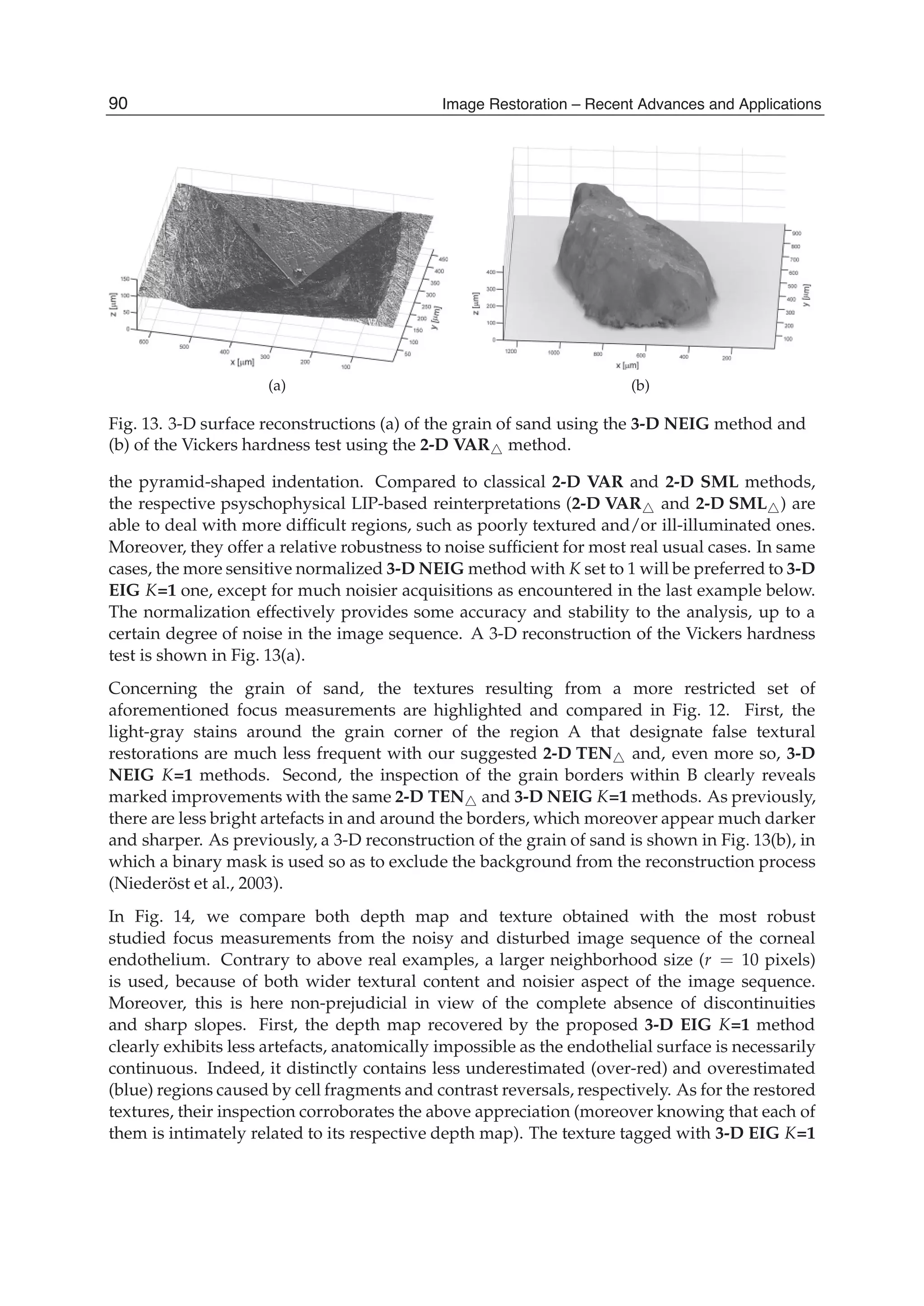
![Surface Topography and Texture Restoration from Sectional Optical Imaging by Focus Analysis 11
1 2 3
4 5 6
7 8 9
1
2
3
4
6
7
8
9
5
Multivariate data matrix
Cross sectional responses
Sectionalobservations
Original sequence of images
1
2
3
4
6
7
8
9
5
1
2
3
4
6
7
8
9
5
1
2
3
4
6
7
8
9
5
1
2
3
4
6
7
8
9
5
1 2 3
4 5 6
7 8 9
1 2 3
4 5 6
7 8 9
1 2 3
4 5 6
7 8 9
1 2 3
4 5 6
7 8 9
z
z
z
z
z
z z z z z
(a)
Cross sectional responses
First eigenvector g
Canonical basis
z
z
z
z
z
(b)
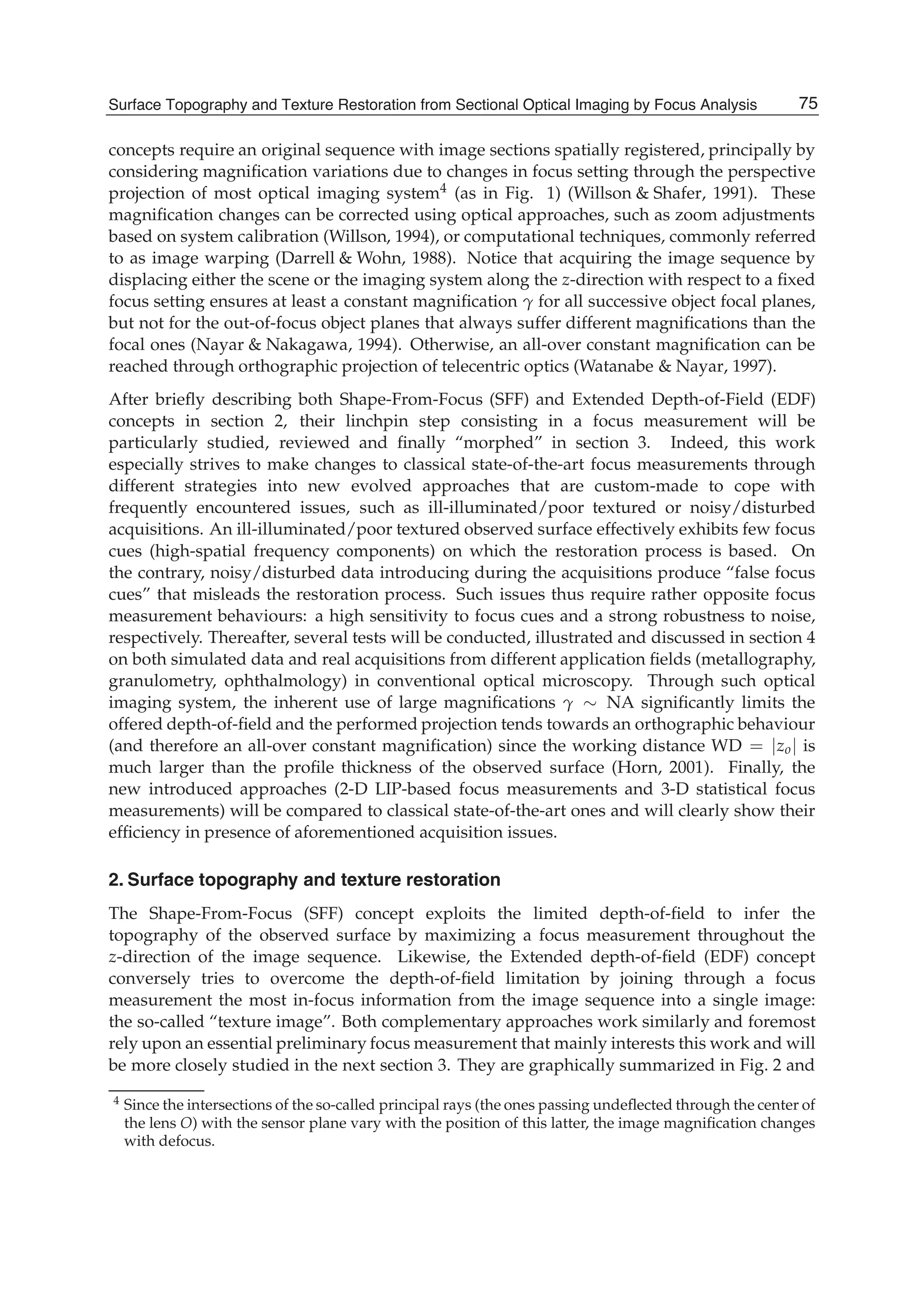
Fig. 5. Illustrations for the 3-D EIG and 3-D N-EIG statistical focus measurements: (a)
creation of the multivariate data matrix X, (b) canonical basis vs. eigenbasis.
where Fmax is the saturating light intensity level (“glare limit”) (Pinoli, 1997b). First, Weber
described the human visual detection between two light intensity values F and G with a
“just noticeable difference”. The LIP subtraction f − g is consistent with Weber’s law (Pinoli,
1997b). In fact, the LIP model defines specific operations acting directly on the physical
light intensity function (stimulus) through the gray tone function notion. A few years after
Weber, Fechner established logarithmic relationship between the light intensity F (stimulus)
and the subjectively perceived brightness B (light intensity sensation). It has been shown
in Pinoli (1997b) that B is an affine map of the isomorphic transform ϕ( f ) of the gray tone
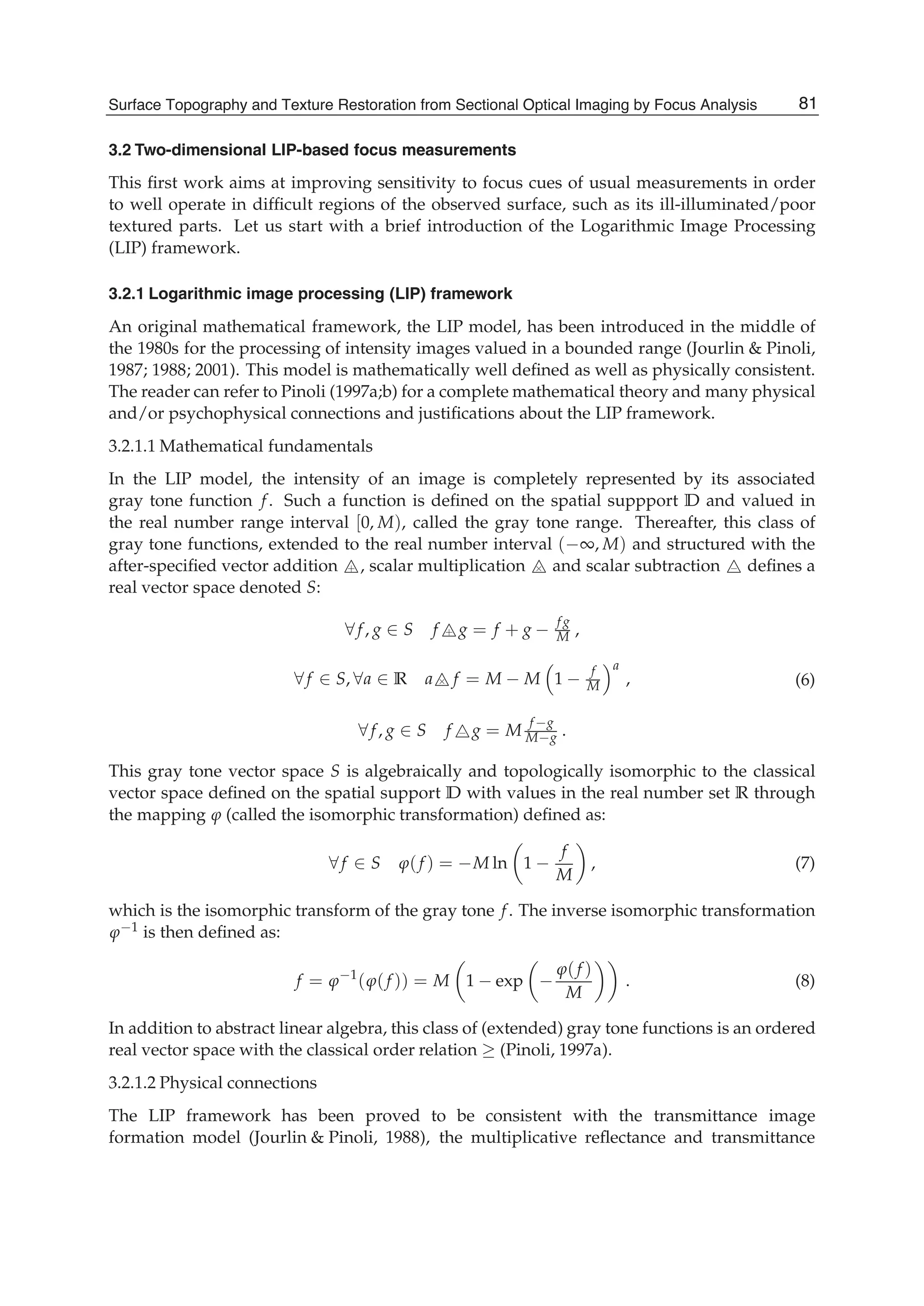
f . Consequently, the fundamental isomorphism ϕ (Eq. 7) of the LIP model should enable
to deal with brightness (via the usual operations). About human brightness perception,
the aforegiven practical limitation accordingly results in revisited measurements attempting
to estimate degree of focus in terms of brightness (intensity sensation from physical light
stimuli). Further details about these 2-D LIP-based focus measurements can be found in
Fernandes et al. (2011a).
3.3 Three-dimensional statistical focus measurements
This second work conversely aims at creating novel 3-D focus measurements offering a large
robustness to noise, while preserving a sufficient sensitivity to focus cues (contrary to the 3-D
DCT-PCA method), in order to well operate through noisy/disturbed acquisitions. In spite
of a similar basic tool, the after-described multivariate statistical analyses are totally different
than the state-of-the-art 3-D DCT-PCA method. Moreover, they do not require any previous
transformations or processings.
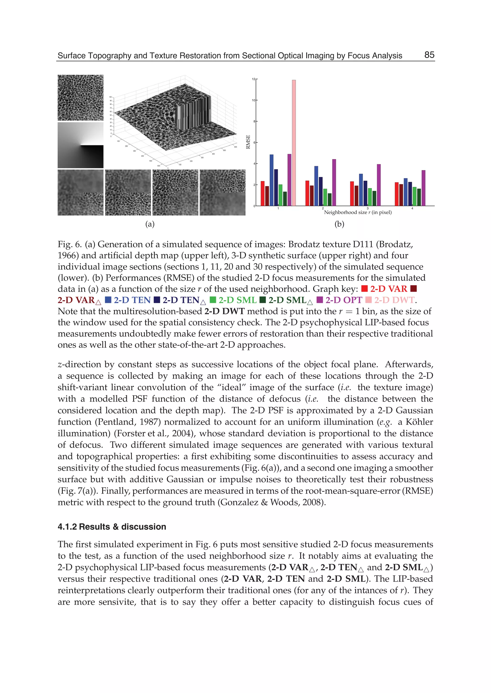
From a stack of single-voxels along the z-direction of the original sequence I(x, y, z) of n
image sections, 2-D sectional windows of m pixels are considered and a multivariate m-by-n
data matrix X is formed as shown in Fig. 5(a). The rows of this data matrix X referred to as the
cross-sectional responses are constituted by the same components of all considered sectional
windows. Let (ei)i∈[1,n] denotes the canonical basis of these cross-sectional responses, whose
each canonical vector ei thus abstracts a different depth zi throughout the image sequence.
Alternatively, each of the columns referred to as the sectional observations fully corresponds
to a different original window at depth z. Note that the variability in variance of these
sectional observations along the z-direction matches with the degree of focus, which is
83Surface Topography and Texture Restoration from Sectional Optical Imaging by Focus Analysis](https://image.slidesharecdn.com/imagerestorationrecentadvancesandapplications-160714160024/75/Image-restoration-recent_advances_and_applications-93-2048.jpg)
![12 Will-be-set-by-IN-TECH
the concept of the traditional 2-D VAR focus measurement. Each sectional observation is
centered, and normalized or not by their means (that will finally yield a couple of different
focus measurements denoted 3-D EIG and 3-D NEIG, respectively). The normalization
enables to locally compensate for differences in intensity means between the image sections of
the sequence. The covariance matrix CX of the sectional observations of X is then calculated
as follows:
CX =
1
m − 1
t
XX , (11)
where t denotes the transpose operation. Afterwards, CX is diagonalized such as:
CXG = ΛG , (12)
in order to obtain both its eigenvalues (λi)i∈[1,n] in increasing order and its eigenvectors
(gi)i∈[1,n], diagonal components and columns of the matrixes Λ and G respectively. The
eigenvectors form a novel orthornormal basis (EIGenbasis) for the cross-sectional responses
of X. Each of them is associated with a particular eigenvalue that reveals its captured
amount of variance among the total one ∑i∈[1,n] λi exhibited by the sectional observations
of X. During the decomposition process of the covariance matrix CX, the first eigenvector g1
accounts for as much of this total variance as possible and the next ones then maximize the
remaining total variance, in order and subject to the orthogonality condition. Furthermore,
less influential noisy information is, to the greatest extent possible, pushed into least dominant
(last) eigenvectors, whereas one of interest remains within the first eigenvectors. Finally, the
degree of focus at the depth zi (with i ∈ [1, n]) is the norm of the orthogonal projection of
the first eigenvector g1 onto the corresponding canonical vector ei, that is simply equal to
the absolute value of the ith component of g1. In the simple schematic example of Fig. 5(b),
the largest degree of focus is clearly assigned to the depth z of index 3 that maximizes the
orthogonal projection norm of the first eigenvector g1. Obviously, several first eigenvectors
can be considered, e.g. the first K eigenvectors, hence the sum of their orthogonal projection
norms respectively weighted by their eigenvalues is regarded. The 3-D EIG and 3-D NEIG
focus analyses then become less robust to noise but relatively gain sensitivity to focus cues.
Further details about these 3-D statistical focus measurements can be found in Fernandes et al.
(2011b; n.d.).
4. Results
Both retained state-of-the-art and novel developed focus measurements will now be
illustrated, tested and compared through various simulation and real experiments.
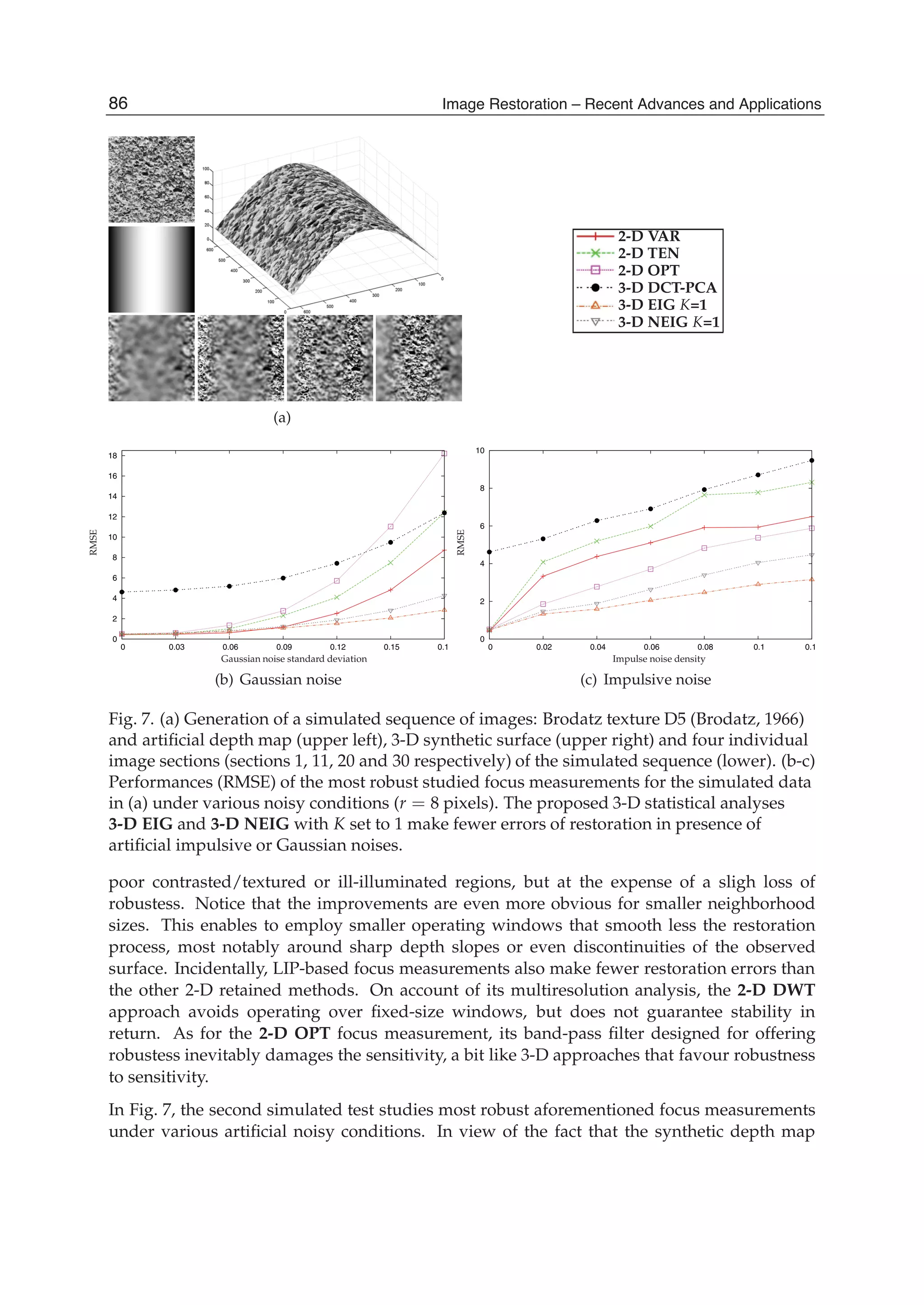
4.1 Performance comparison in simulation
A first serie of experiments using simulated data is conducted in order to dispose of ground
truths for carrying out quantitative assessments of the results produced by all aforementioned
methods.
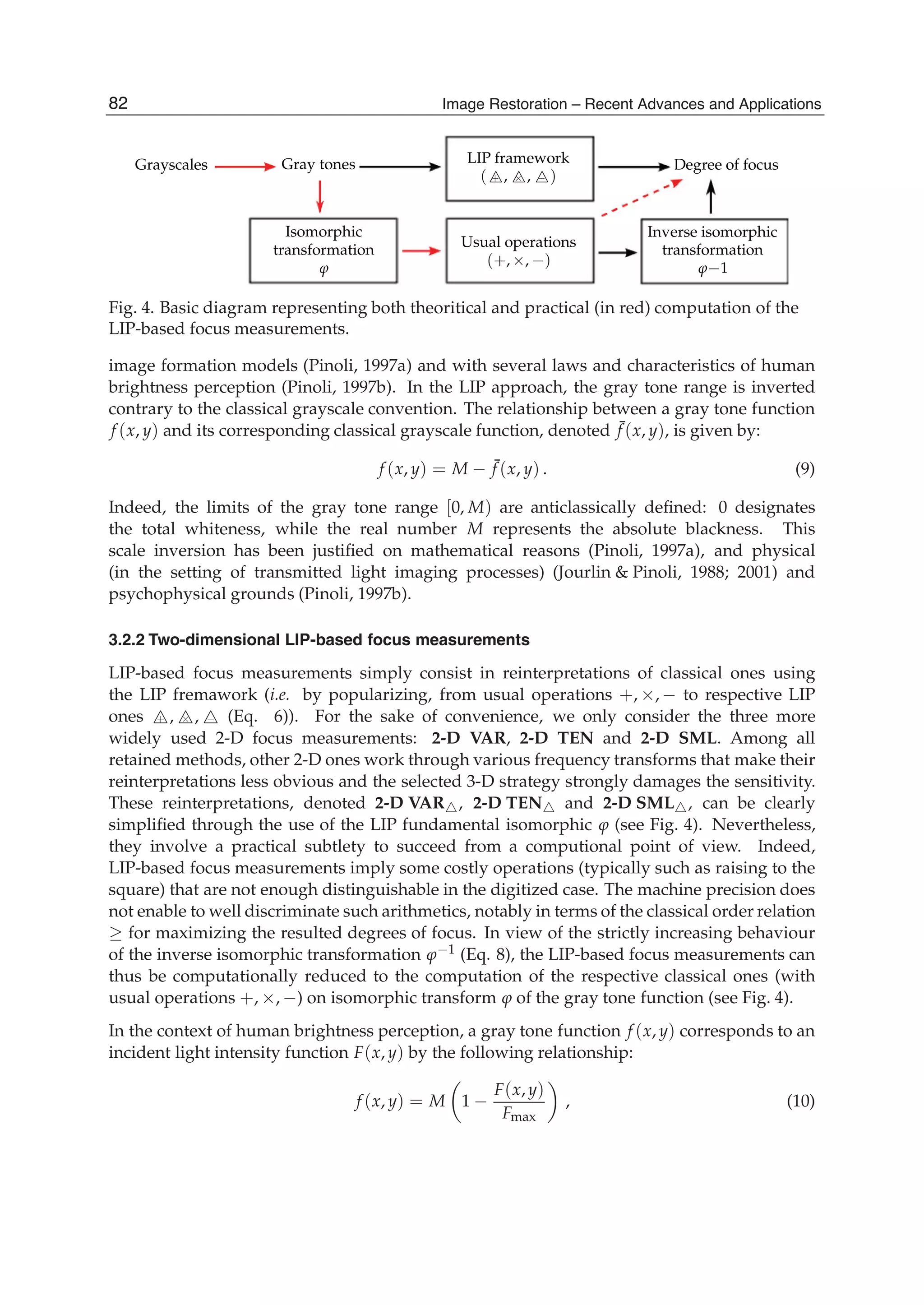
4.1.1 Simulation process & performance assessment
By first mapping an arbitrary texture onto a simulated depth map (that constitutes the ground
truth), an artificial 3-D surface is constructed. This virtual surface is then discretized along the
84 Image Restoration – Recent Advances and Applications](https://image.slidesharecdn.com/imagerestorationrecentadvancesandapplications-160714160024/75/Image-restoration-recent_advances_and_applications-94-2048.jpg)
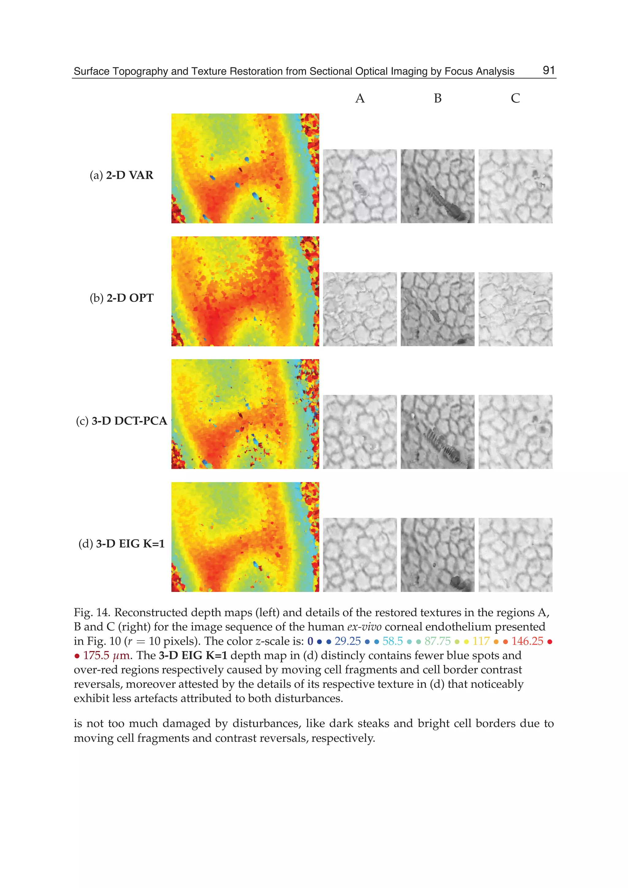


![Defocused Image Restoration with Local Polynomial Regression and IWF 3
by a factor of 2. The l level wavelet decomposition of an image I results in an approximation
image Xl and three detail images Hl, Vl, and Dl in horizontal, vertical, and diagonal directions
respectively. Decomposition into l levels of an original image results in a down sampled image
of resolution 2l with respect to the image as well as detail images.
When an image is defocused, edged in it are smoothed and widened. The amount of high
frequency band decreased, and that corresponding to low frequency band increases.
In order to denote the relationship between wavelet coefficients and defocused radius R, we
define five variables named v1, v2, v3, v4, and v5 as:
⎧
⎪⎪⎪⎪⎪⎨
⎪⎪⎪⎪⎪⎩
v1 = |V2|s/|H2|s
v2 = |H2|s/|X2|s
v3 = |H1|s/num{H1}
v4 = |H2|s/num{H2}
v5 = |D1|s/num{D1}
(4)
where | · |s represents the summation of all coefficients’ absolute value, num{·} is total number
of coefficients.
An original image is blurred artificially by a uniform defocus PSF with R whose value ranging
from 1 to 20. The relationship between v1, v2, v3, v4, v5 and R are shown in Fig.1, where
the curves are normalized in [0,1] interval. When R increases, v2, v3, v4 and v5 decrease
monotonously.
0 5 10 15 20
0
0.2
0.4
0.6
0.8
1
cameraman
v1
v2
v3
v4
v5
0 5 10 15 20
0
0.2
0.4
0.6
0.8
1
rice
v1
v2
v3
v4
v5
Fig. 1. Relationship Between v1−5 and R
In order to estimate defocus parameter R, only known the roughly similar relationship is not
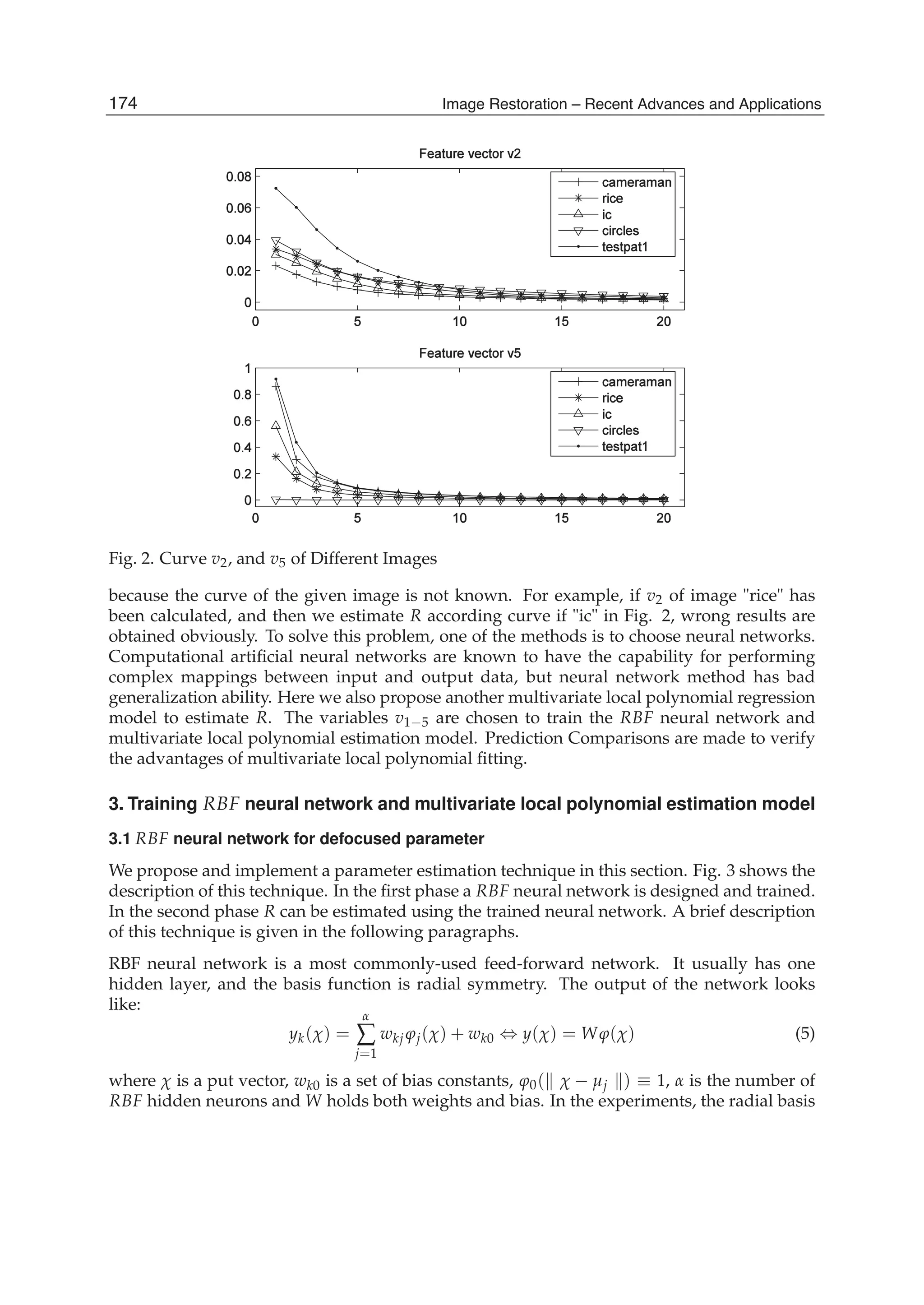
enough. As shown in Fig. 2, every image has monotonous curve between v2, v5 and R, but
they are not superposition. For a degraded unknown PSF image, R can not be calculated
173Defocused Image Restoration with Local Polynomial Regression and IWF](https://image.slidesharecdn.com/imagerestorationrecentadvancesandapplications-160714160024/75/Image-restoration-recent_advances_and_applications-183-2048.jpg)
![Defocused Image Restoration with Local Polynomial Regression and IWF 5
Fig. 3. Defocus Parameter Estimation Process
functions are chosen as of Gaussian type:
ϕj( χ − μj ) = exp[−
1
2γ2
j
χ − μj
2
] (6)
where μj is the center and γj is the standard deviation of the Gaussian function, respectively.
Sixteen original images are chosen to train the RBF net. The images are defocused artificially
with R whose value ranging from 2 to 7. So the total number of training samples are 96. Then
feature vectors are constructed using variables p1−5 of each image:
χ = (p1, p2, p3, p4, p5) (7)
For the network output vector, we use one-of-k encoding method, that is, for R =2, t =
(0, 0, 0, 0, 0, 1)T; for R = 3, t = (0, 0, 0, 0, 1, 0)T, and so on.
When training samples {χi, ti}96
i=1 are given, the weights matrix W can be obtained as W =
TΦ†, Φ† is pseudo-inverse of Φ, where Φ is a matrix:
Φ =
⎛
⎜
⎜
⎜
⎝
1 · · · 1
ϕ(||χ1 − μ1||) · · · ϕ(||χ96 − μ1||)
...
...
...
ϕ(||χ1 − μα||) · · · ϕ(||χ96 − μα||)
⎞
⎟
⎟
⎟
⎠
(8)
and T = (t1, t2, · · · , t96).
After obtaining weights matrix W, the defocused parameter R can be calculated using the
trained RBF network.
175Defocused Image Restoration with Local Polynomial Regression and IWF](https://image.slidesharecdn.com/imagerestorationrecentadvancesandapplications-160714160024/75/Image-restoration-recent_advances_and_applications-185-2048.jpg)
![Defocused Image Restoration with Local Polynomial Regression and IWF 7
The localization scheme at a point x assigns the weight
KH(Xi − x), with KH(x) = |H|−1
K(H−1
x), (14)
where |H| is the determinant of the matrix H. The bandwidth matrix is introduced to
accommodate the dependent structure in the independent variables. For practical problems,
the bandwidth matrix H is taken to be a diagonal matrix. The different independent variables
will be accommodated into different scales. For simplification, the bandwidth matrix is
designed into H = hIm (Im denoting the identity matrix of order m).
3.2.2 Multivariate predictor with local polynomial fitting
Suppose that the input vector is V = (v1, v2, v3, v4, v5). The model is fitted by the function
R = f (V). (15)
Our purpose is to obtain the estimation ˆR = ˆf (V) of function f . This paper, we use the dth
order multivariate local polynomial f (V) to predict the defocused parameter RT value based
on the point VT of the test image. The polynomial function can be described as
f (V) ≈ ∑
0≤|j|≤d
1
j!
D(j)
fi(VT)(V − VT)j
= ∑
0≤|j|≤d
bj(VT)(V − VT)j
(16)
where
m = 5, j = (j1, j2, · · · , jm), j! = j1!j2! · · · jm!, |j| =
m
∑
l=1
jl, (17)
∑
0≤|j|≤d
=
d
∑
|j|=0
(
|j|
∑
j1=0
|j|
∑
j2=0
· · ·
|j|
∑
jm=0
)
|j|=j1+j2+···+jm
, Vj
= v
j1
1 v
j2
2 · · · v
jm
m , (18)
D(j)
fi(VT) =
∂|j|
fi(V)
∂v
j1
1 ∂v
j2
2 · · · ∂v
jm
m
|V=VT
, bj(VT) =
1
j!
D(j)
fi(VT). (19)
In the multivariate prediction method, VTa
(a = 1, 2, · · · , A) denoting the trained image feature
vectors. Using A pairs of (VTa
, Ra), for which the values are already known, the coefficients of
fi is determined by minimizing
A
∑
a=1
[Ra − ∑
0≤|j|≤d
bj(VT)(VTa
− VT)j
]2
· KH(VTa
− VT) (20)
For the weighted least squared problem, a matrix form can be described by
W1/2
· Y = W1/2
· X · B + ε (21)
where
Y = (y1, y2, · · · , yA)T
, ya = Ra, (22)
B = (b0(VT), b1(VT), · · · , bd(VT))T
, (23)
177Defocused Image Restoration with Local Polynomial Regression and IWF](https://image.slidesharecdn.com/imagerestorationrecentadvancesandapplications-160714160024/75/Image-restoration-recent_advances_and_applications-187-2048.jpg)
![Defocused Image Restoration with Local Polynomial Regression and IWF 9
Another issue in multivariate local polynomial fitting is the choice of the order of the
polynomial. Since the modeling bias is primarily controlled by the bandwidth, this issue is
less crucial however. For a given bandwidth h, a large value of d would expectedly reduce the
modeling bias, but would cause a large variance and a considerable computational cost. Since
the bandwidth is used to control the modeling complexity, and due to the sparsity of local
data in multi-dimensional space, a higher-order polynomial is rarely used. We use the local
quadratic regression to indicate the flavor of the multivariate local polynomial fitting, that is
to say, d = 2.
The third issue is the selection of the kernel function. In this paper, of course, we choose the
optimal spherical Epanechnikov kernel function, which minimizes the asymptotic MSE of the
resulting multivariate local polynomial estimators, as our kernel function.
3.2.4 Estimating the defocused parameter
Twenty original images are chosen to train the model. The images are defocused artificially
with R whose value ranging from 2 to 7. So the total number of training samples are 120. Then
feature vectors are constructed using variables v1−5 of each image:
V = (v1, v2, v3, v4, v5) (30)
The defocused parameters R is the model output.
When training samples {VTa
, Ra}120
a=1 are given, obtaining weights matrix B, according to the
relationship between the V and R, then the defocused parameter R can be calculated using
the trained model.
4. Iterative Wiener filter
Wiener filtering (minimizing mean square error ) is commonly used to restore
linearly-degraded images. To obtain optimal results,there must be accurate knowledge of
the covariance of the ideal image. In this section, the so-called iterative Wiener filter Su et al.
(2008); Allen et al. (1990)is used to restore the original image.
The imaging system H is assumed to be linear shift invariant with additive, independent,
white noise processes of known variance. the model for the observed image y is given in
matrix notation by
y = H f + n (31)
where f is the ideal image. The optimal linear minimum mean-squared error, or Wiener
restoration filter given by
ˆf = By (32)
where B = Rf f HT[HRf f HT + Rnn]−1, requires accurate knowledge of Rf f , the
autocorrelation of ideal image f. However, in practical situations f is usually not available
and only a single copy of the blurred image to be restored, y, is provided. In the absence
of a more accurate knowledge of the ideal image f, the blurred image y is often used in its
place simply because there is no other information about f readily available. The signal y is
subsequently used to compute an estimate of Rf f and this estimate is used in place of Rf f in
Equation (32).
The following summarizes the iterative Wiener filtering procedure.
179Defocused Image Restoration with Local Polynomial Regression and IWF](https://image.slidesharecdn.com/imagerestorationrecentadvancesandapplications-160714160024/75/Image-restoration-recent_advances_and_applications-189-2048.jpg)
![10 Image Restoration
step 1 Initialization: Use y to compute an initial (i=0) estimate of Rf f by
Rf f (0) = Ryy = E{yyT
} (33)
Step 2 Filter construction: Use Rf f (i), the ith estimate of Rf f to construct the (i + 1)th
restoration filter B(i + 1) given by
Bi+1 = Rf f HT
[HRf f HT
+ Rnn]−1
(34)
Step 3 Restoration: Restore y by the B(i + 1) filter to obtain ˆf (i + 1), the (i + 1)th estimate of f
ˆf (i + 1) = B(i + 1)y (35)
Step 4 Update: Use ˆf (i + 1) to compute an improved estimate of Rf f , given by
Rf f (i + 1) = E{ ˆf (i + 1) ˆf T
(i + 1)} (36)
Step 5 Iteration: Increment i and repeat steps 2,3,4, and 5.
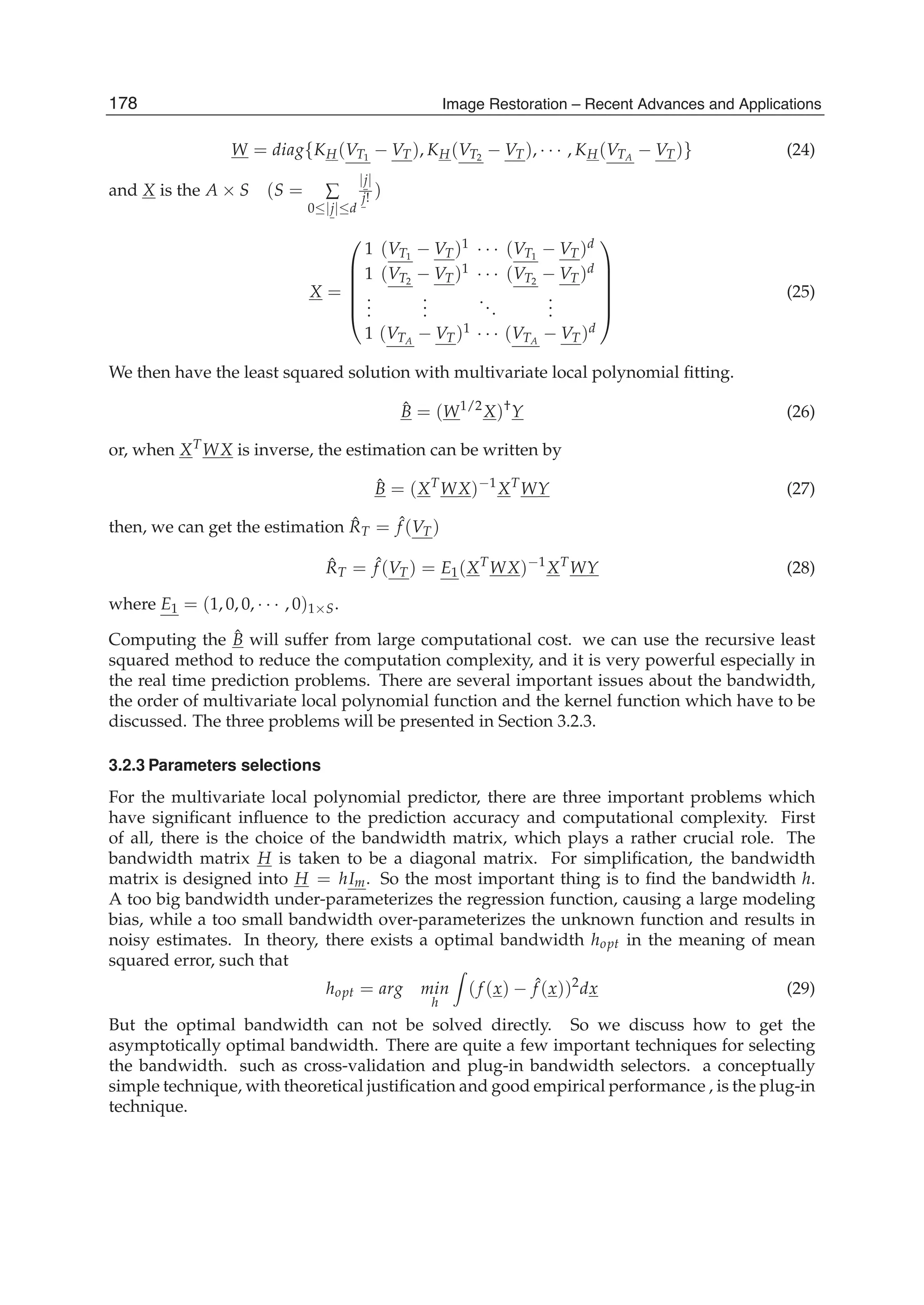
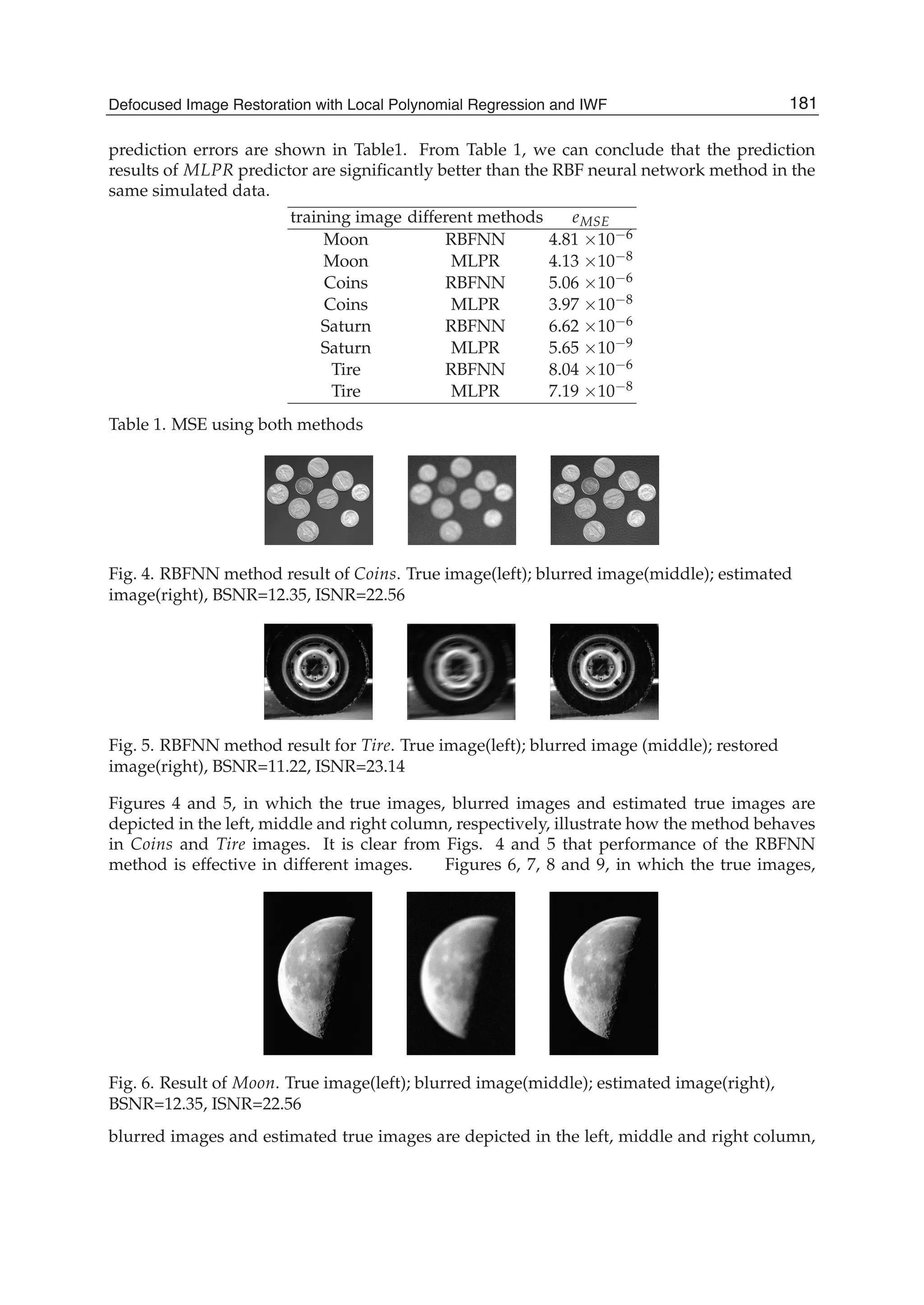
5. Experimental results and analysis
The experiments are carried out by using the Matlab image processing toolbox. The
performance of the proposed image restoration algorithm has been evaluated using the
classical gray-scale Moon image, Coins image, Saturn image, and Tire image in Matlab
toolbox. To verify the good ability of restoration of the proposed algorithm, one real blurred
image is used for the deconvolution procedure. The results show our method is very
successful for this kind of blurred image.
In image restoration studies, the degradation modelled by blurring and additive noise is
referred to in terms of the metric blurred signal-to-noise ratio (BSNR). This metric for a
zero-mean M × N image is given by
BSNR = 10log10{
1
MN ∑M
m=1 ∑N
n=1 z2(m, n)
σ2
v
} (37)
where z(m, n) is the noise free blurred image and σ2
v is the additive noise variance.
For the purpose of objectively testing the performance of linear image restoration algorithms,
the improvement in signal-to-noise ratio (ISNR) is often used. ISNR is defined as
ISNR = 10log10{
∑M
m=1 ∑N
n=1[f (m, n) − y(m, n)]2
∑M
m=1 ∑N
n=1[f (m, n) − ˆf (m, n)]2
} (38)
where f (m, n) and y(m, n) are the original and degraded image pixel intensity values and
ˆf (m, n) is the restored true image pixel intensity value. ISNR cannot be used when the true
image is unknown, but it can be used to compare different methods in simulations when the
true image is known.
In order to find the good performance of the proposed multivariate local polynomial
Regression method (MLPR) compared with the RBF neural network algorithm (RBFNN) Su
et al. (2008), the same defocused blurred images are used for the experiments. Mean squared
180 Image Restoration – Recent Advances and Applications](https://image.slidesharecdn.com/imagerestorationrecentadvancesandapplications-160714160024/75/Image-restoration-recent_advances_and_applications-190-2048.jpg)
![Image Restoration Using Two-Dimensional Variations 187
where is a parameter of regularization. Note that the statistical methods used in image
restoration lead to optimization problems, which are similar to that of Eq. (3). For instance,
using Bayes’ strategy (Kay, 1993) we can obtain the optimal estimation in the following form:
*
2 1inf{ ln ( ) ln ( )}
z Z
z p Az v p z
, (4)
where 1( )p and 2( )p are a priori probability densities of the original image z and
additive noise .n Az v The main difference between the regularization method of image
restoration in Eq. (3) and the statistical method in Eq. (4) is the regularization parameter .
This leads to a family of solutions as a function of the parameter . The best restored image
can be chosen from the set of solutions using, for instance, a subjective criterion. If the space
Q in Eq. (3) is the Euclidian space with the norm (v, Bv), where B is a positive defined
operator, we obtain,
2*
inf{ ( )}Bz Z
z Az v z
. (5)
It is commonly assumed that the original image is a smooth function with respect to the
Sobolev space (Adams, 1975), and the stabilization functional in Eq. (5) is ( ) p
q
q
W
z z .
Quadratic forms can be used in order to avoid nonlinear restoration algorithms. Note that a
Gaussian image model leads to minimization of a quadratic form. In discrete case it
corresponds to the Sobolev norm for 2p in Eq. (5). On the other hand, the use of
quadratic forms in image restoration often yields undesirable results because of real images
are not Gaussian. Now suppose that an image to be restored is a function of bounded
variations. Therefore, it may be written as
*
inf{ ( , ) ( )}Q
z Z
z Az v Var z
. (6)
The variation of a 1D function ( ), [ , ]f x x a b is defined as follows:
1....
1
2
( ) sup ( ) ( )
n
nb
k k
a x x k
V f f x f x
. (7)
It can be shown, that if the image ( , )z x y , ( , )x y D consists of 1D functions of bounded
variation along its rows and columns then the image is also a 2D function of bounded
variation. Different multidimensional variations were proposed such as variations of Arzela,
Vitali, Tonelly, etc. (Vitushkin, 1955). A different approach was suggested by Kronrod, who
introduced two functionals in order to describe an image as a function of two variables
(Kronrod, 1950). The functionals are given as follows:
1 0( ) ( )td z m e dt
, and 2 1( ) ( )td z m e dt
, (8)
where te is t - level set of the function ( , )z x y , i.e. a set of points ( , )x y with function values
equal to t, 0( )tm e is the number of components of te , and 1( )tm e is the length of the set te .](https://image.slidesharecdn.com/imagerestorationrecentadvancesandapplications-160714160024/75/Image-restoration-recent_advances_and_applications-197-2048.jpg)
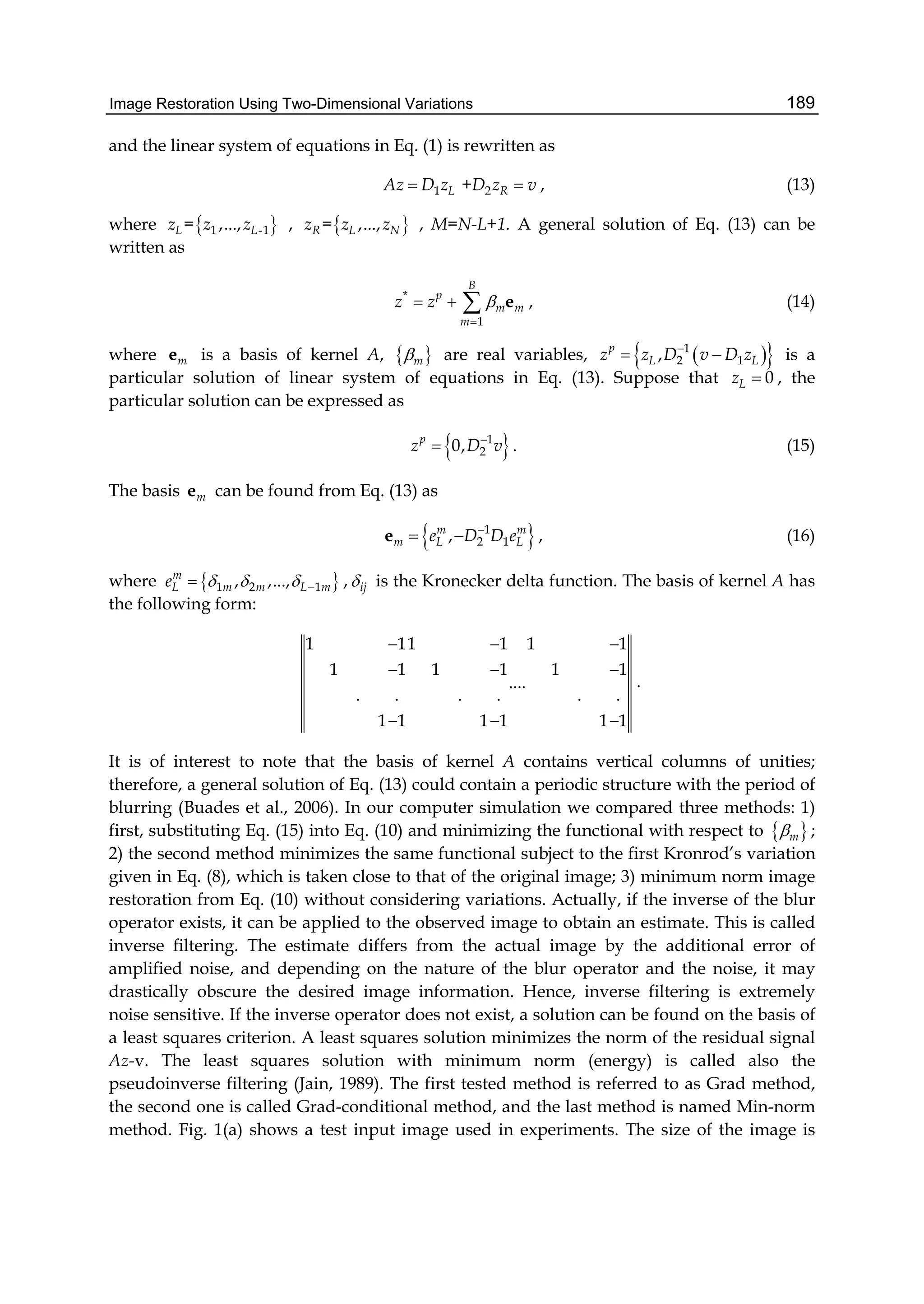
![Image Restoration – Recent Advances and Applications190
256×256 pixels, N=256. The signal range is [0-255]. The test input scene is homogeneously
blurred with L=7. The blurred image is shown in Fig. 1(b).
(a)
(b)
Fig. 1. (a) Test image, (b) test image uniformly blurred in horizontal direction with L=7.
The original image has the following values of the Kronrod variations: d1=2105, d2=12210.
The results of image restoration with the variation methods are shown in Figs. 2(a) and 2(b),
respectively. The restoration result with the Min-norm algorithm is shown in Fig. 2(c).
Subjective visual criterion is defined as an enhanced difference between original and
restored images. A pixel is displayed as gray if there is no error between the original image
and the restored image. For maximum error, the pixel is displayed either black or white
(with intensity values of 0 and 255, respectively).](https://image.slidesharecdn.com/imagerestorationrecentadvancesandapplications-160714160024/75/Image-restoration-recent_advances_and_applications-200-2048.jpg)
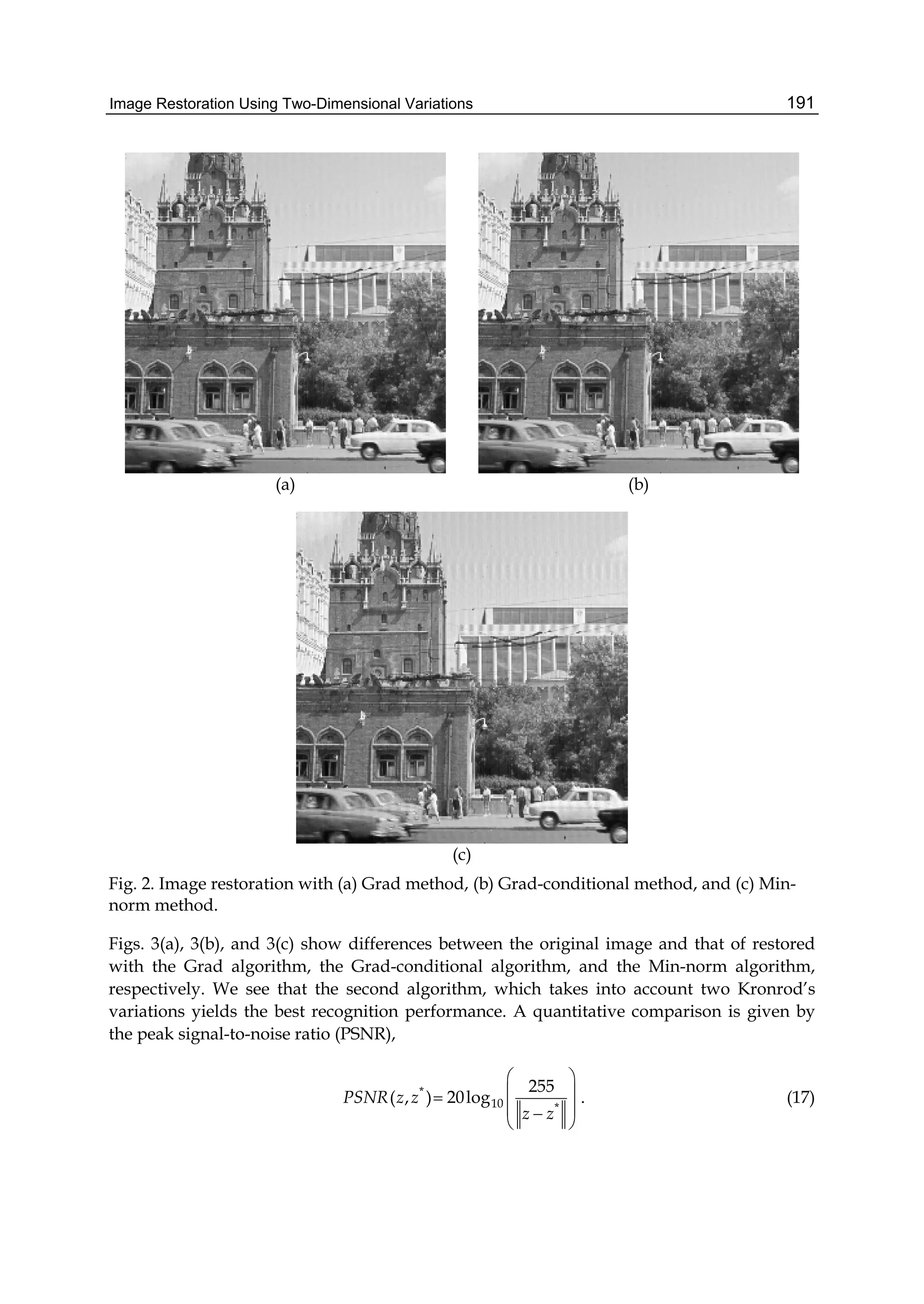
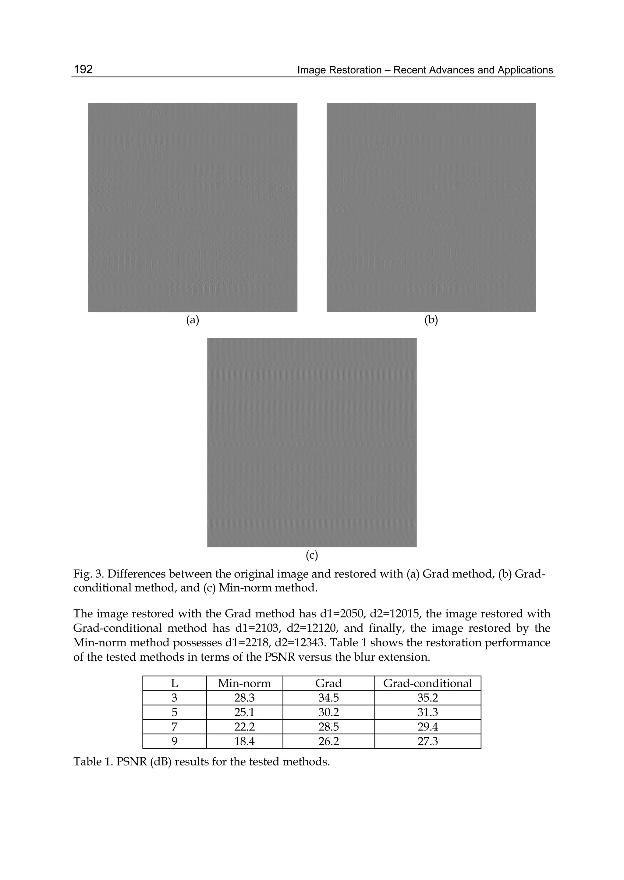
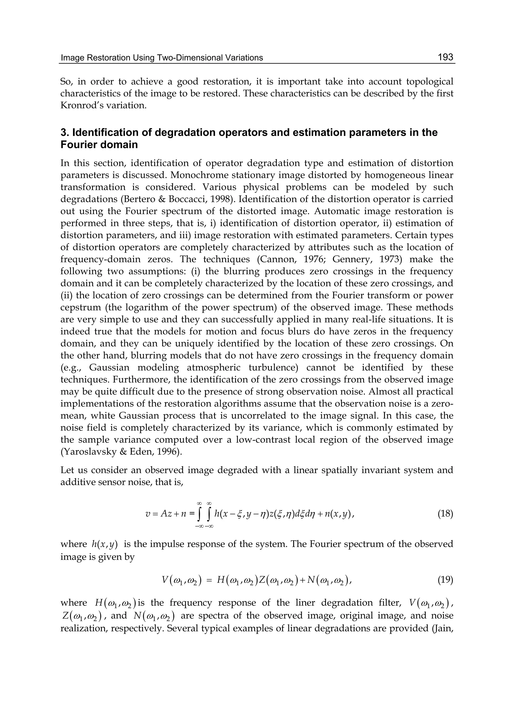
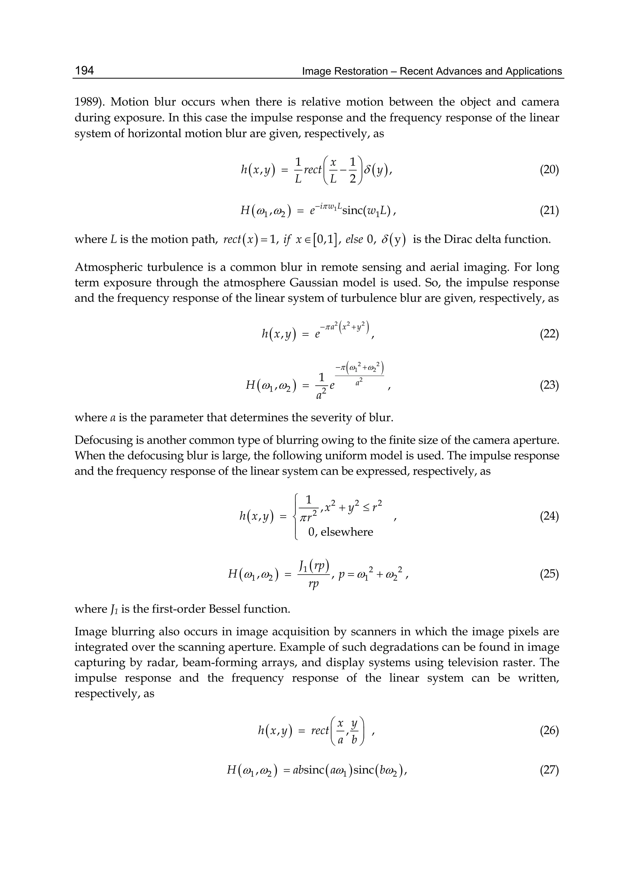
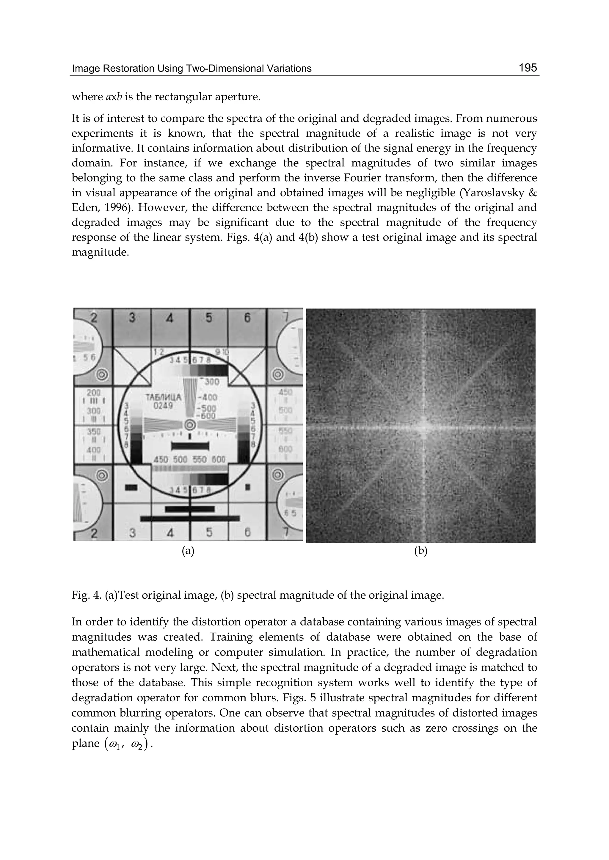
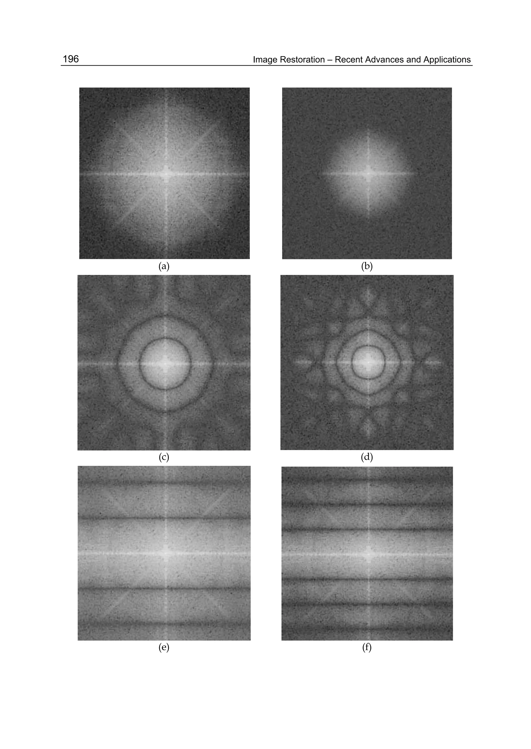
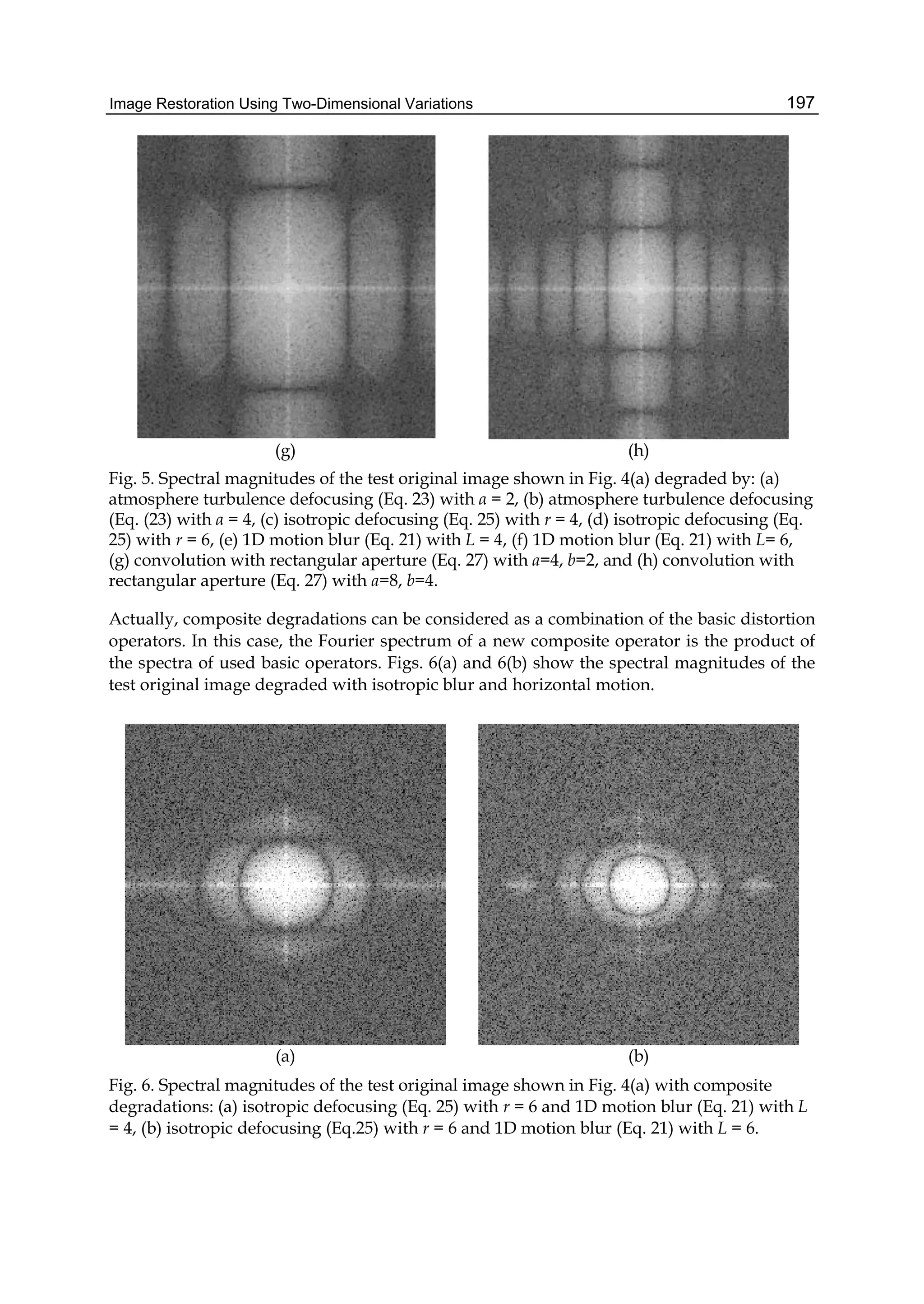
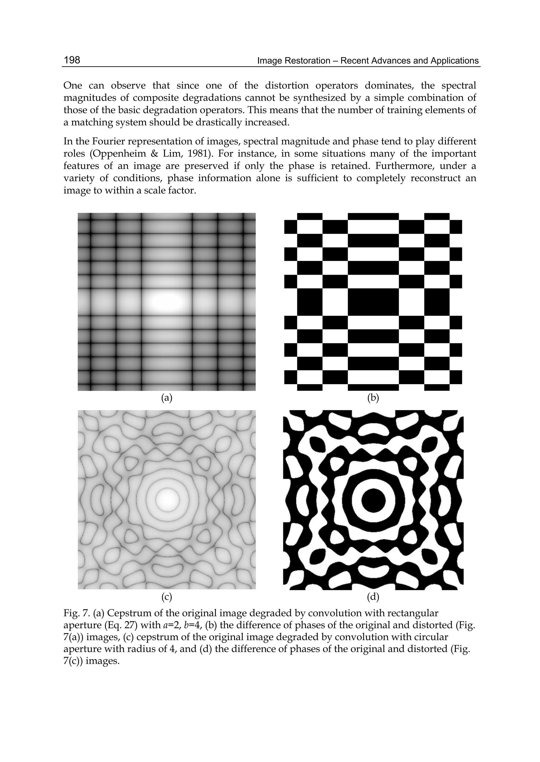
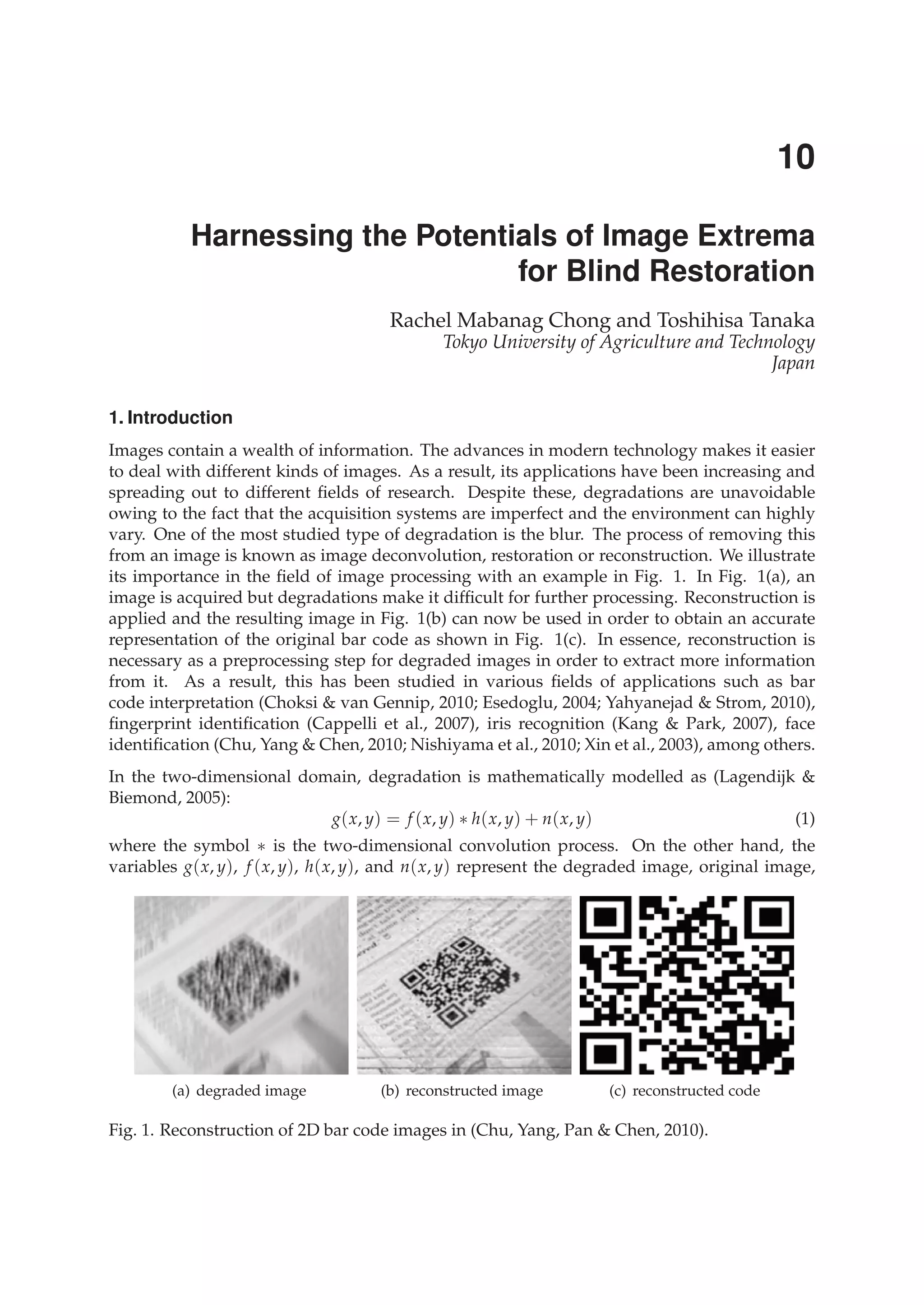
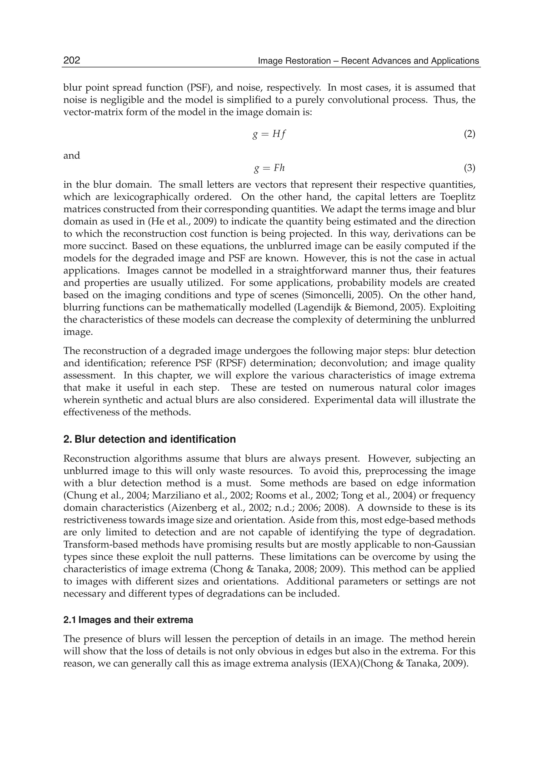
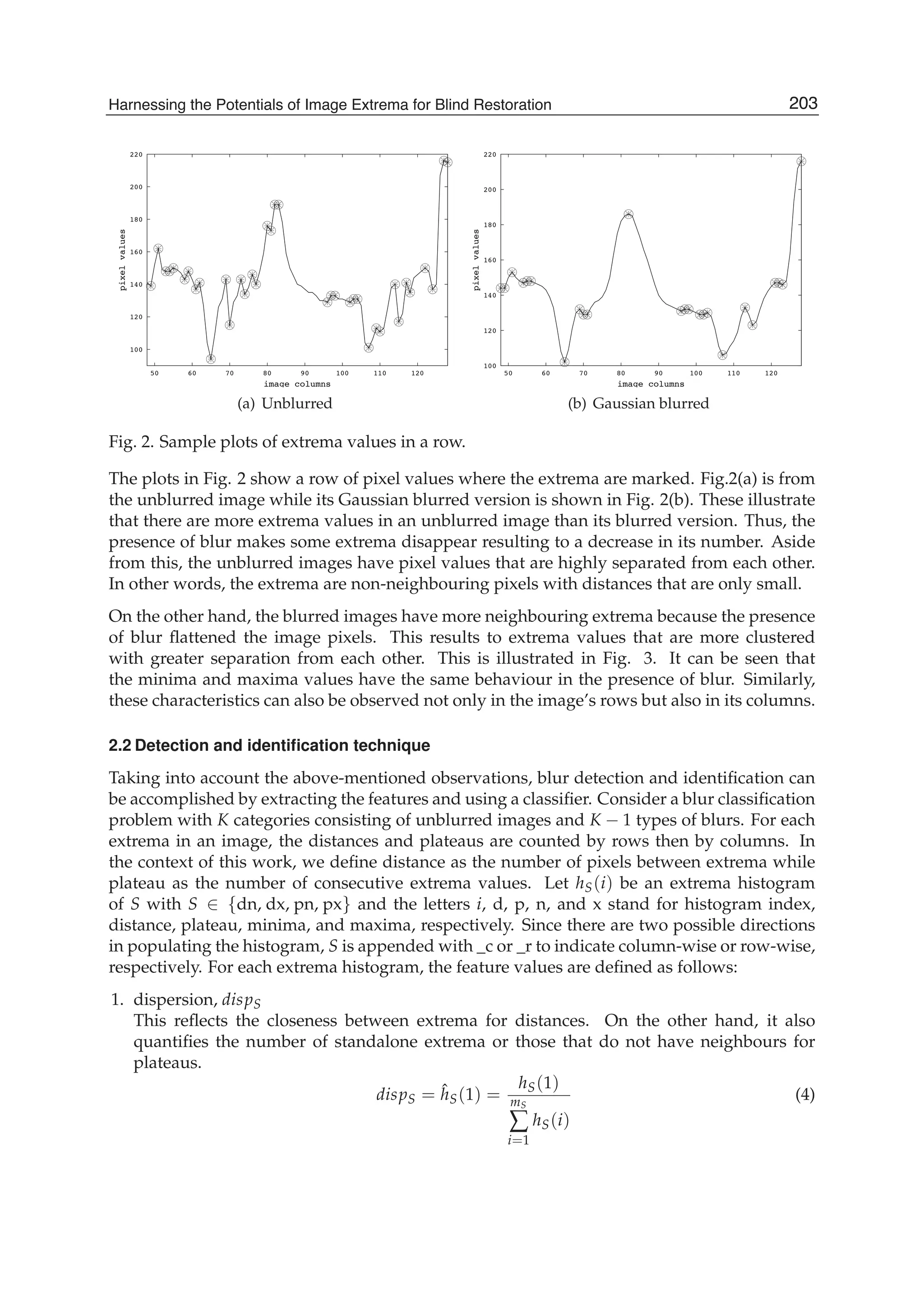
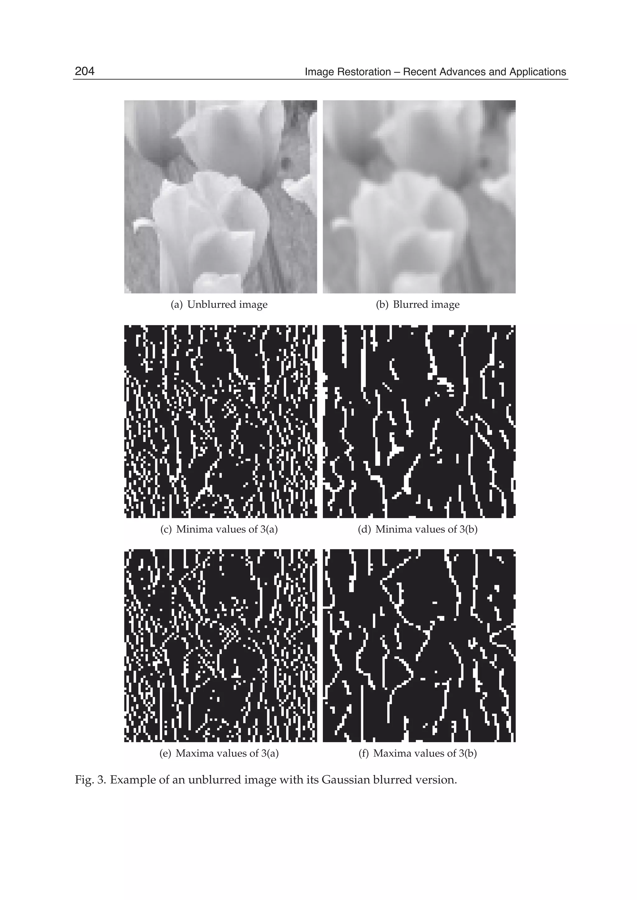
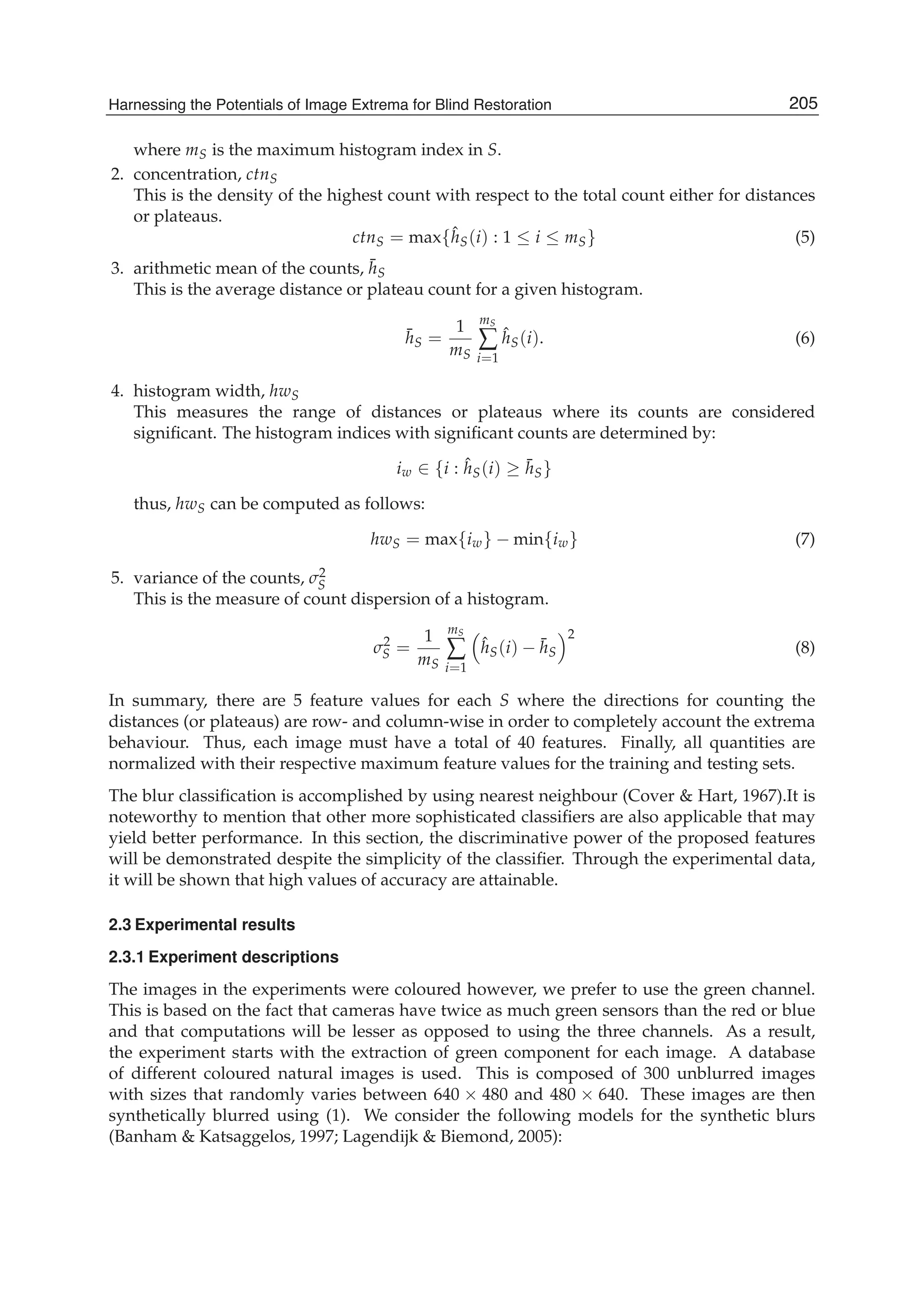
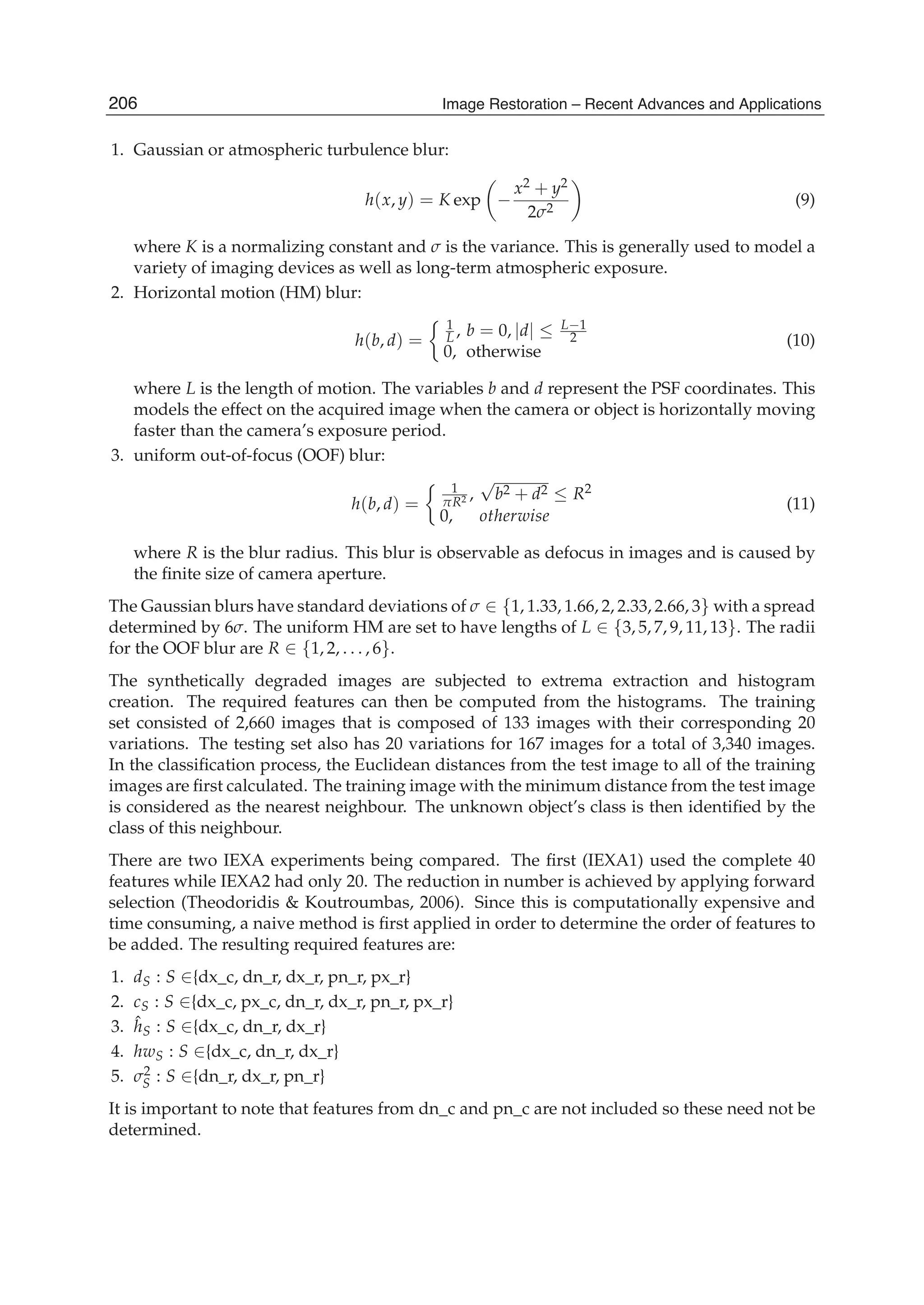
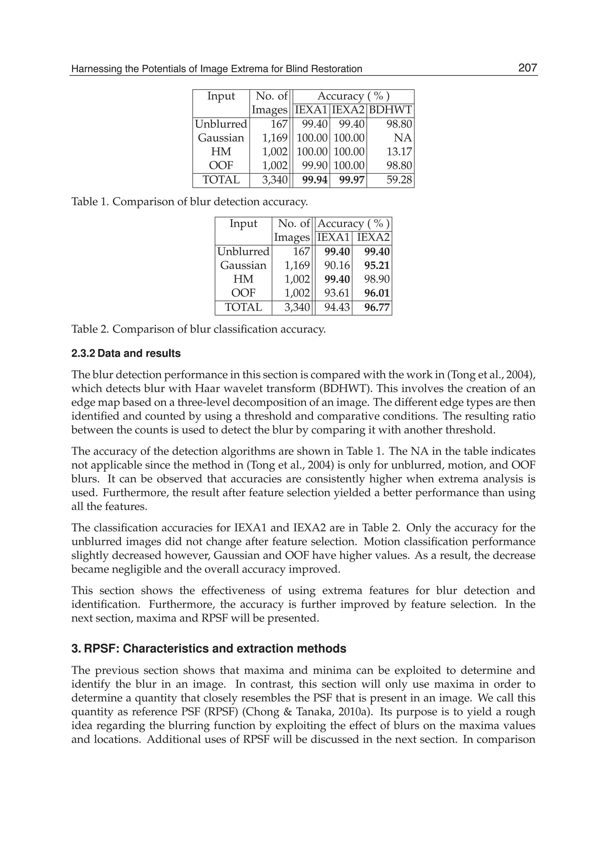
![8 Will-be-set-by-IN-TECH
with the previous section, this does not require a classifier or image features. It is extracted
from the given image assuming only a PSF size.
3.1 Motion blurs and maxima
The presence of blur has the effect of flattening the pixel values. As a result, the locations
of the maxima values are influenced by the blurring function. In (Chong & Tanaka, 2010a;
2011b) the extraction of RPSF has been tested on motion and OOF blurred images. However,
the most commonly encountered type of blur is motion. Thus, more focus will be given to this
type. In this case we will consider the general model of the motion blur given by:
h(b, d; L, θ) =
1
L ,
√
b2 + d2 ≤ L
2 and b
d = − tan θ
0, otherwise
(12)
where the parameter θ represents motion angle in degrees.
Figure 4 shows images blurred by motion in different directions. Each degraded image
consists of two maxima images based on the direction of scanning. These are shown as binary
images in Figs. 4(c)-4(f) where the white pixels indicate the maxima. It can be observed that
the locations are influenced by the direction of motion that is present. As a result, the maxima
locations tend to be arranged in the direction of motion. Considering a small window in the
image where the maxima are present, it is obvious that this will give us an idea regarding
the direction of motion. This is indicated by the larger pixel values located at the direction
of motion. To detect the direction Hough transform has been utilized in (Chong & Tanaka,
2010b; 2011a). In image processing, this is commonly used to detect lines and circles in binary
images. For a straight line, all of its points will intersect in the parameter space [(Gonzales &
Woods, 2008)]. The parameters (ζ and θ) are specified from the representation of a line in the
PSF space domain:
b cos θ + d sin θ = ζ (13)
where parameter θ can be interpreted as the direction of motion. Since the PSFs are discrete
and have sizes smaller than the image, the parameter space can be easily subdivided. For
practical purposes, we set θ = {0◦, 45◦, 90◦, 135◦}. The accumulator for a certain combination
of ζ and θ is incremented based on the point located at (b, d). The detection of the motion
direction is accomplished by selecting the accumulator with the maximum number of points.
3.2 RPSF extraction
The RPSF can be extracted from motion blurred images by the following steps:
1. Scan the green channel of the image for local maxima locations in the horizontal and
vertical directions.
2. Determine the number of locations for each scanning direction and let Z be the total count.
3. If z is the index of the maxima locations and assuming a blur support size of s × s, create
a set of windows {wz}Z
z=1 of the same size whose elements are the pixel values with the
maxima value at the center.
4. Compute the sum of these windows by
w = ω
Z
∑
z=1
wz. (14)
208 Image Restoration – Recent Advances and Applications](https://image.slidesharecdn.com/imagerestorationrecentadvancesandapplications-160714160024/75/Image-restoration-recent_advances_and_applications-218-2048.jpg)
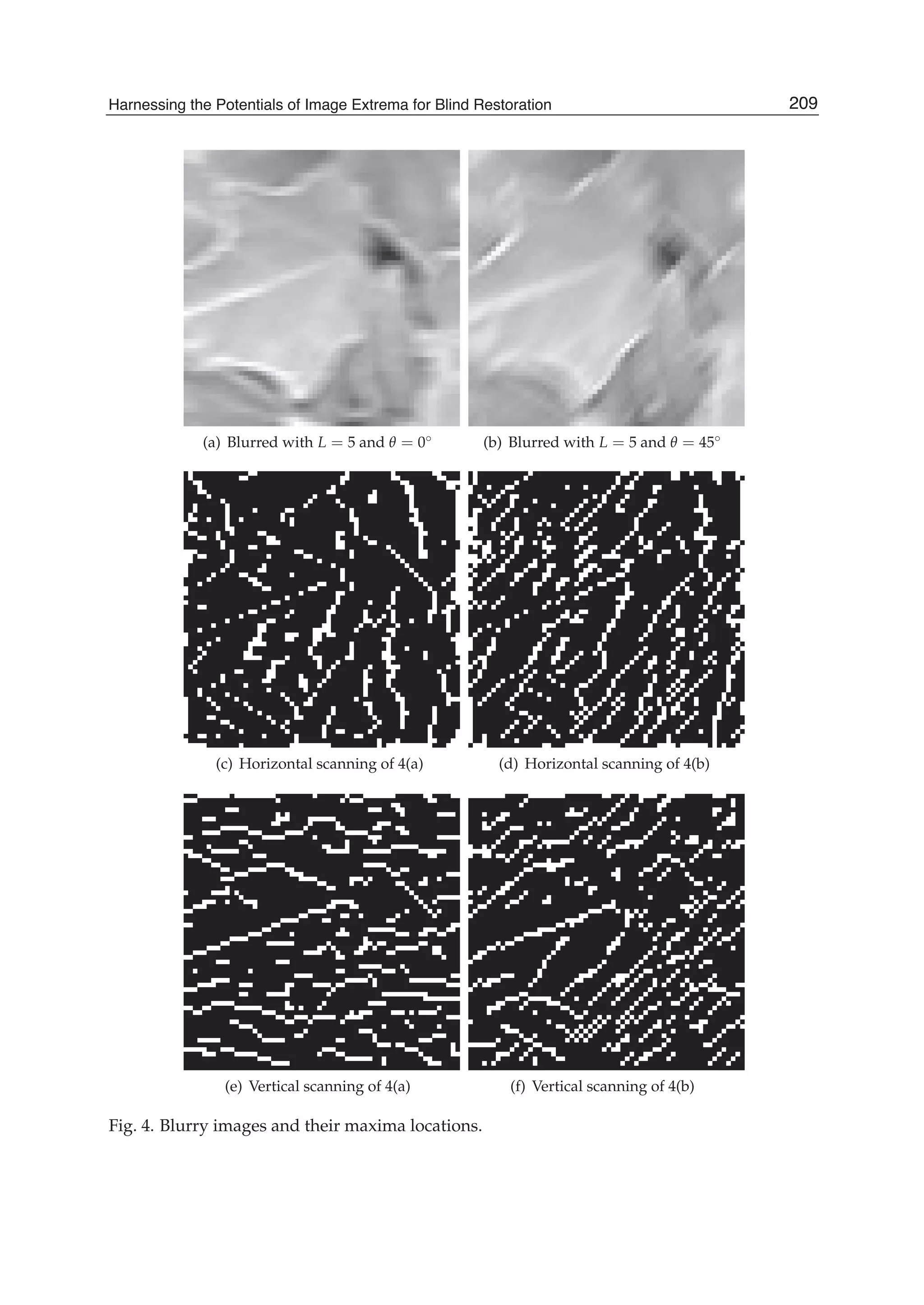
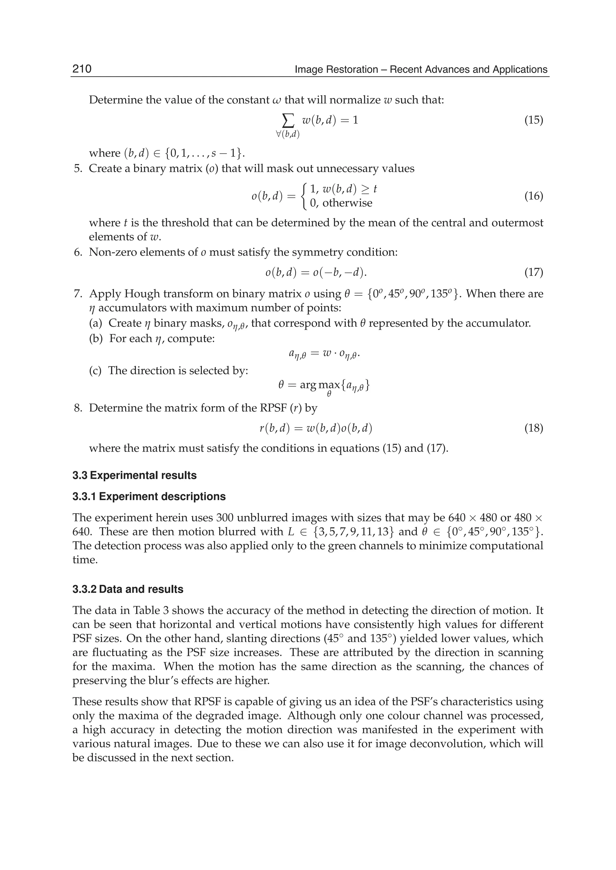
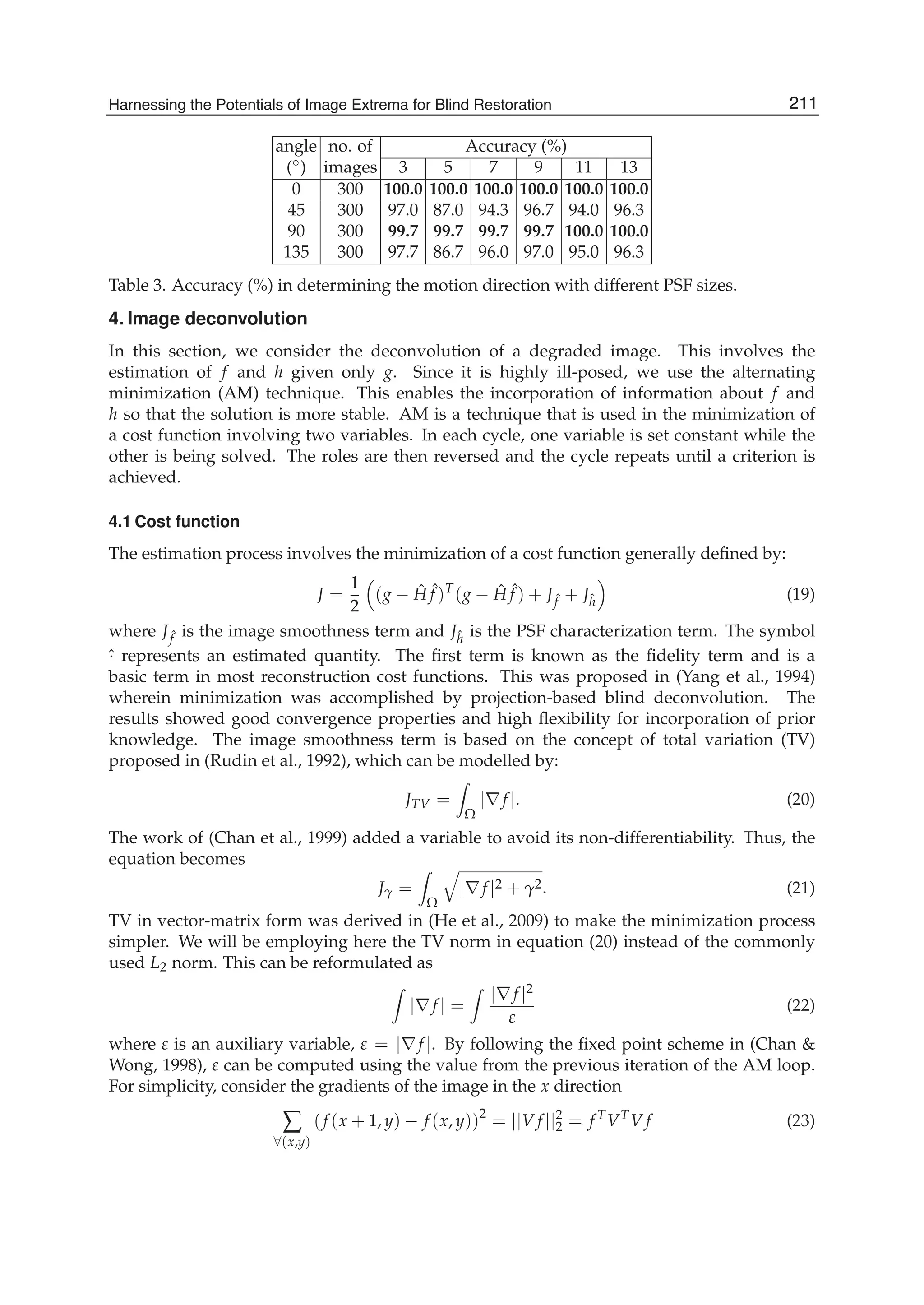
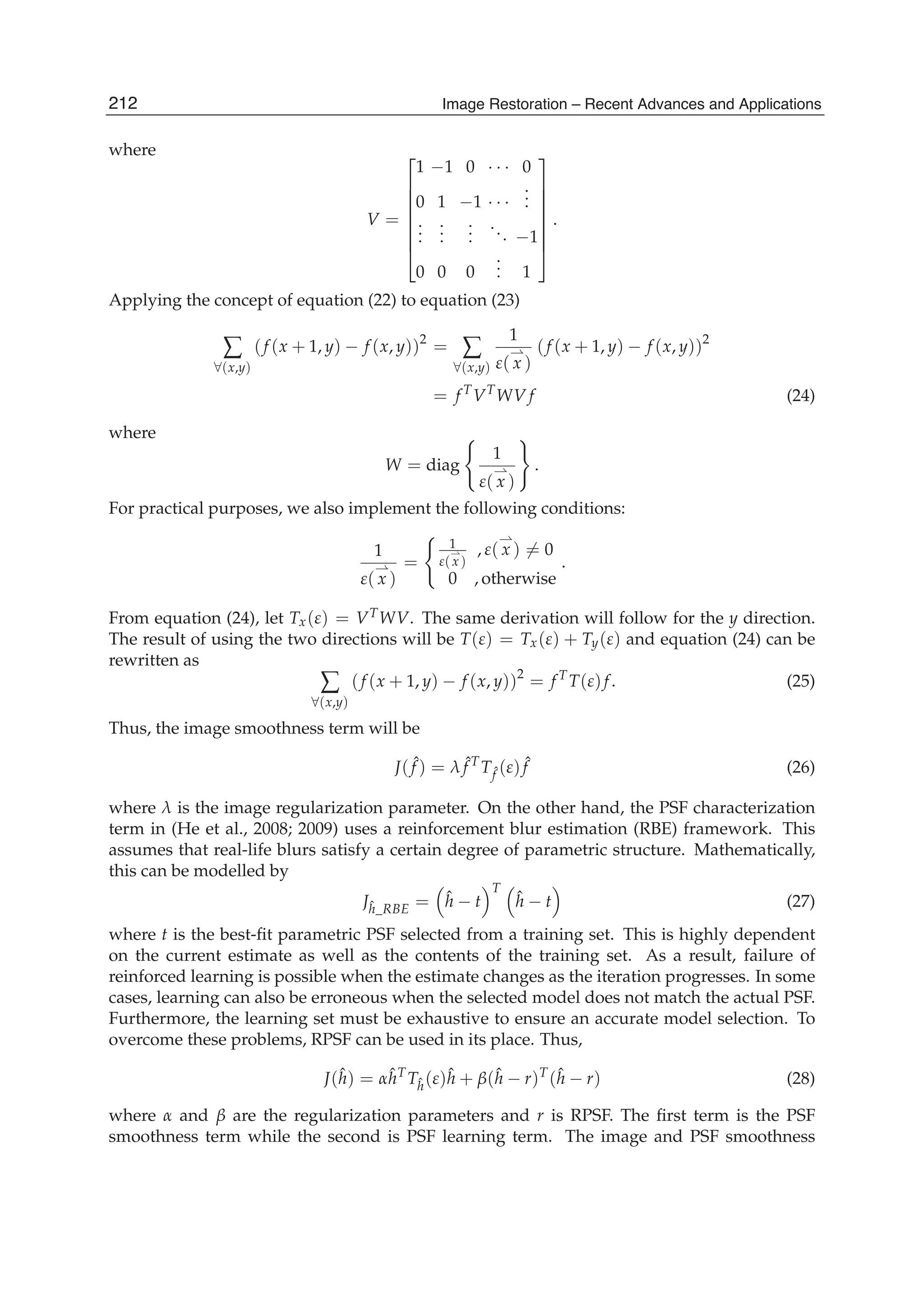
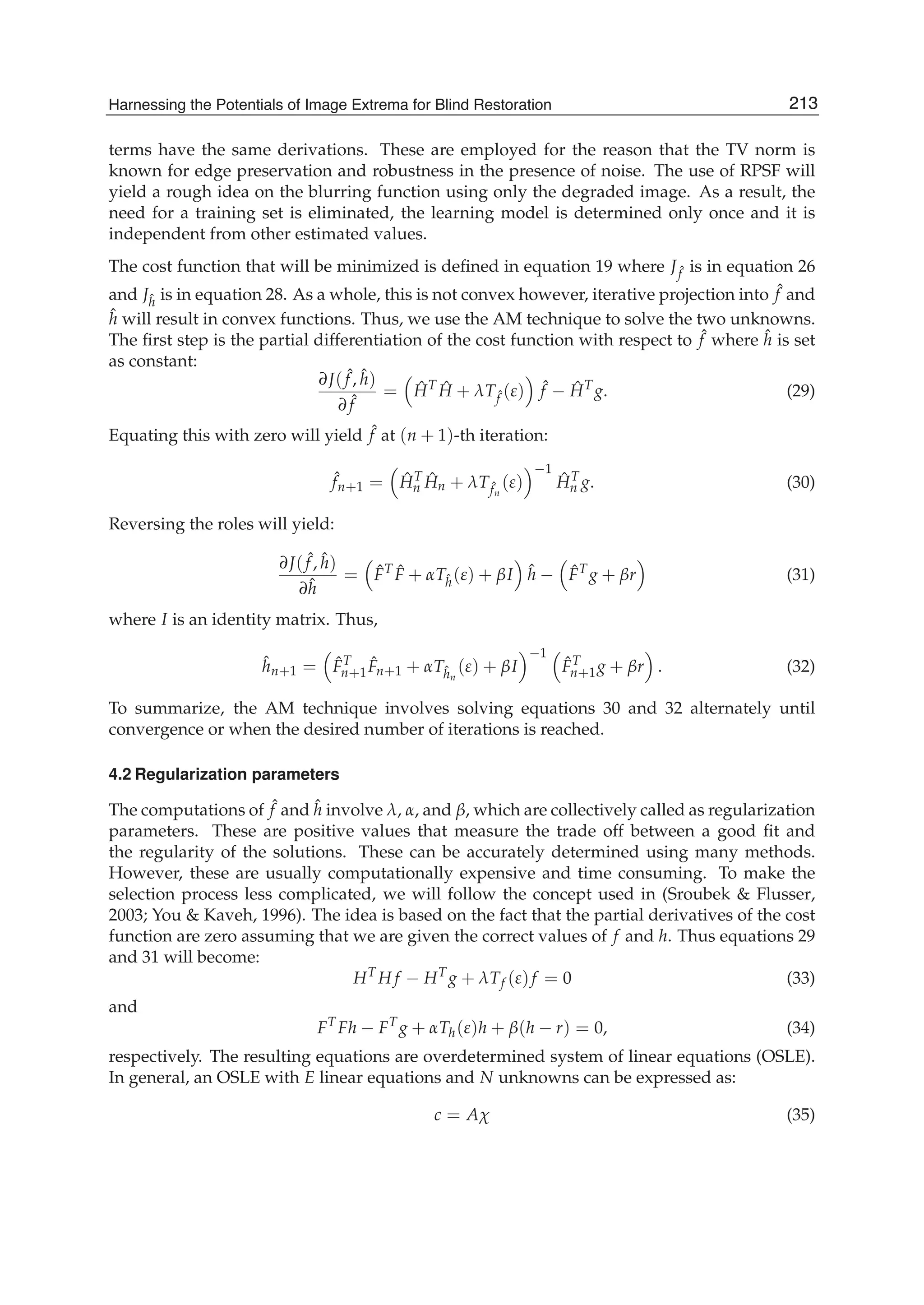
![14 Will-be-set-by-IN-TECH
where c is a vector of given values with c ∈ E×1 , A is a matrix of coefficients with A ∈ E×N,
and χ is a vector of unknown variables with χ ∈ N×1. Using minimum sum of squared error
approximation (Cadzow, 2002), the solution can be determined by:
χ = (AT
A)−1
AT
c. (36)
Based on equation 33, λ can then be computed by:
λ = (AT
f Af )−1
AT
f cf (37)
where Af = −Tf (ε)f and cf = HT H f − HT g. Similarly, α and β can be solved from equation
34:
[ α β ]T
= (AT
h Ah)−1
AT
h ch (38)
where Ah = −[Th(ε)h (h − r)] and ch = FT Fh − FT g.
In practical applications, the correct values of f and h are unknown. The estimated values, ˆf
and ˆh, may be utilized in lieu of the unknown correct values then equations 37 and 38 can be
used to compute approximate values of the regularization parameters. In this case, parameter
tuning is done iteratively with a stopping criterion that may be based on the maximum PSNR;
a fixed iteration count; or the minimum cost function, among others.
4.3 Experimental results
4.3.1 Experiment descriptions
The experiment in this section will investigate the effects of integrating the RPSF during the
deconvolution of synthetically blurred images. An unblurred image shown in Fig. 5(c) has
a size of 60 × 60 pixels. This is synthetically blurred with a PSF defined by equation 10 with
the following parameters: L ∈ {3, 5, 7} and θ ∈ {0◦, 45◦, 90◦, 135◦}. The unblurred image and
PSF are known thus, the results can be easily monitored and verified. In this way, a reference
can be established for cases when both the unblurred image and PSF are unknown.
The regularization parameters are computed for 50 iterations. The selection is based on the
maximum peak signal-to-noise ratio (PSNR) in dB, which can be computed as follows:
PSNRdB = 10 log10
2b − 1
2
MSE
(39)
where MSE is defined by
MSE =
1
XY ∑
∀(x,y)
f (x, y) − ˆf (x, y)
2
(40)
and b is the number of bits used to represent a pixel value. The selected parameters are shown
in Table 4. Using these values, ˆf and ˆh are computed for 20 iterations. The initial estimated
image is equated to the given degraded image while the PSF is composed of positive real
random numbers.
The quality of the estimated image is quantitatively evaluated by computing its PSNR. On
the other hand, the estimated PSF is compared with the actual PSF by mean squared error
214 Image Restoration – Recent Advances and Applications](https://image.slidesharecdn.com/imagerestorationrecentadvancesandapplications-160714160024/75/Image-restoration-recent_advances_and_applications-224-2048.jpg)
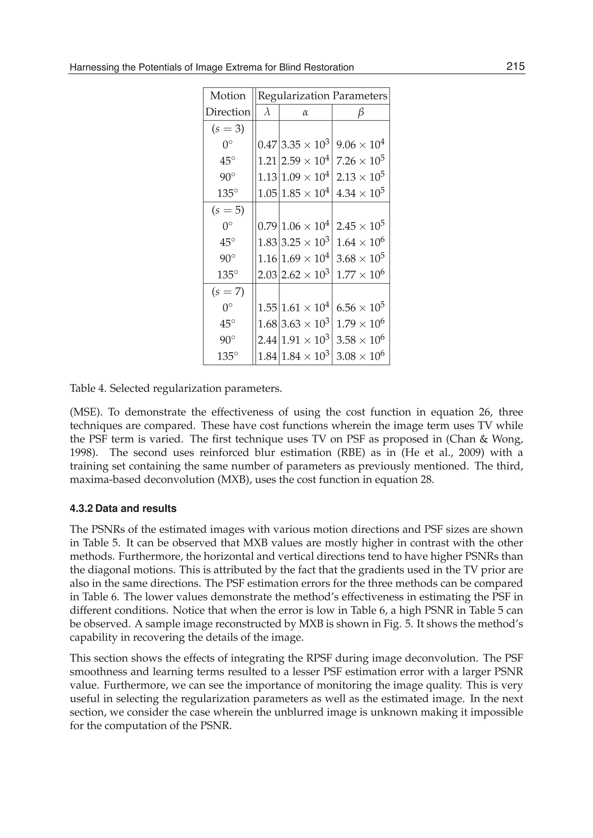
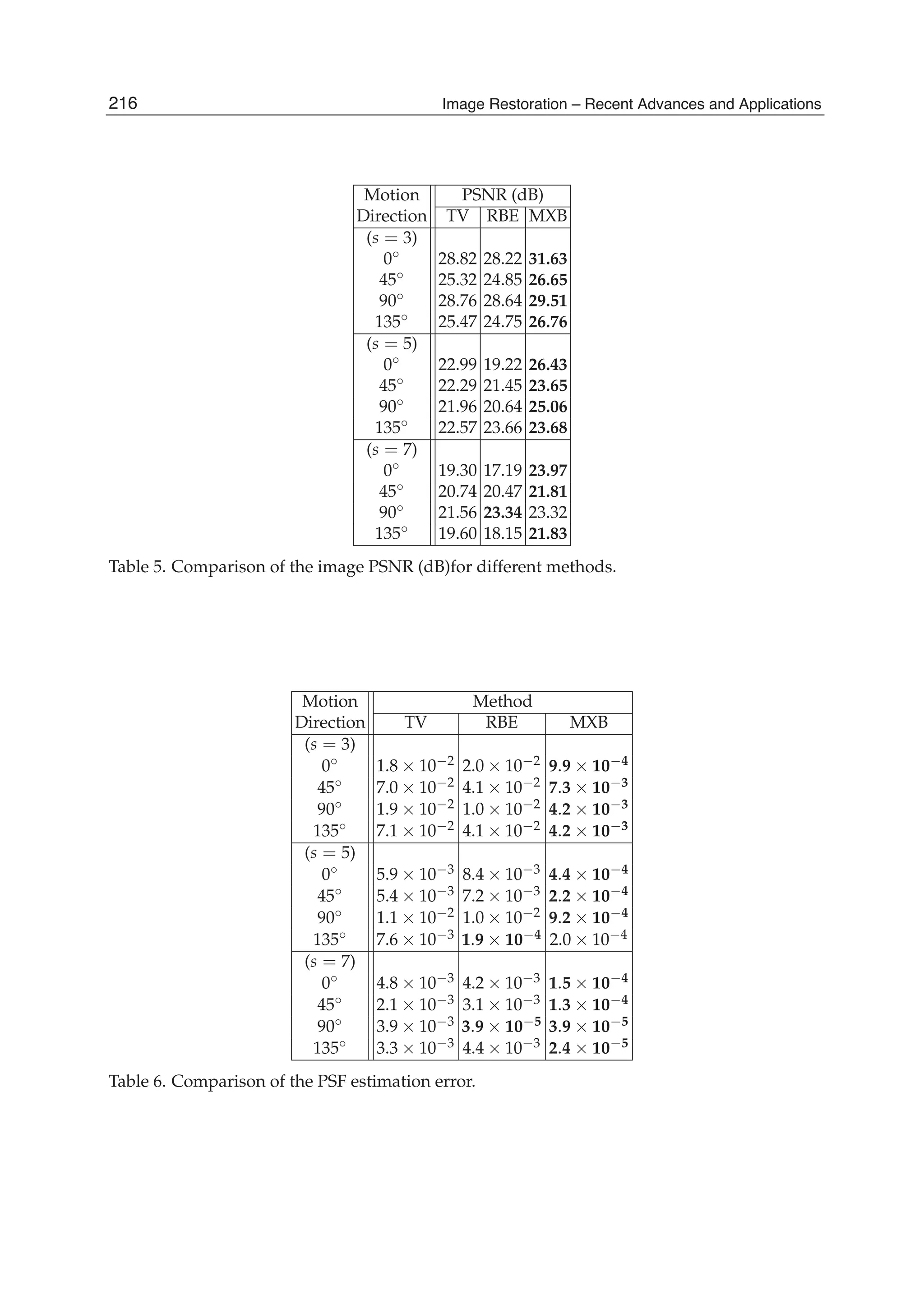
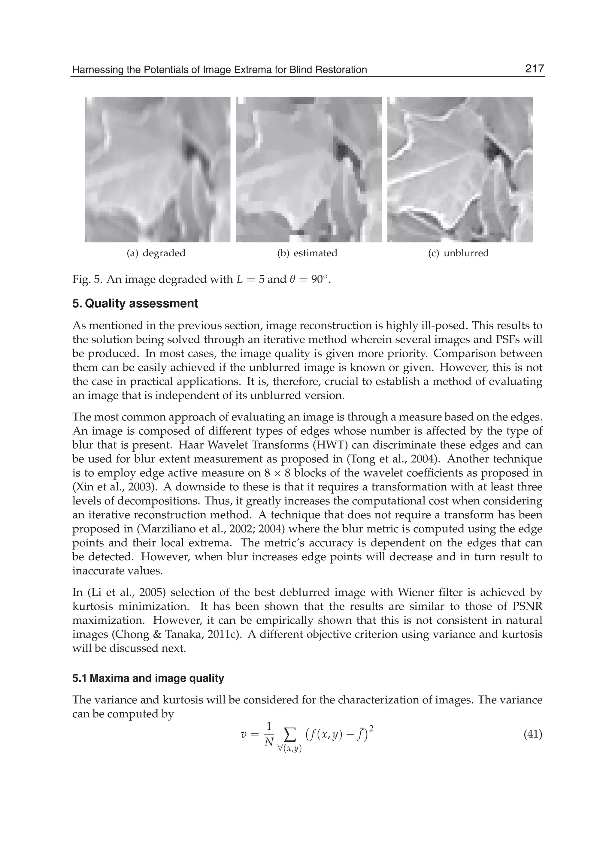
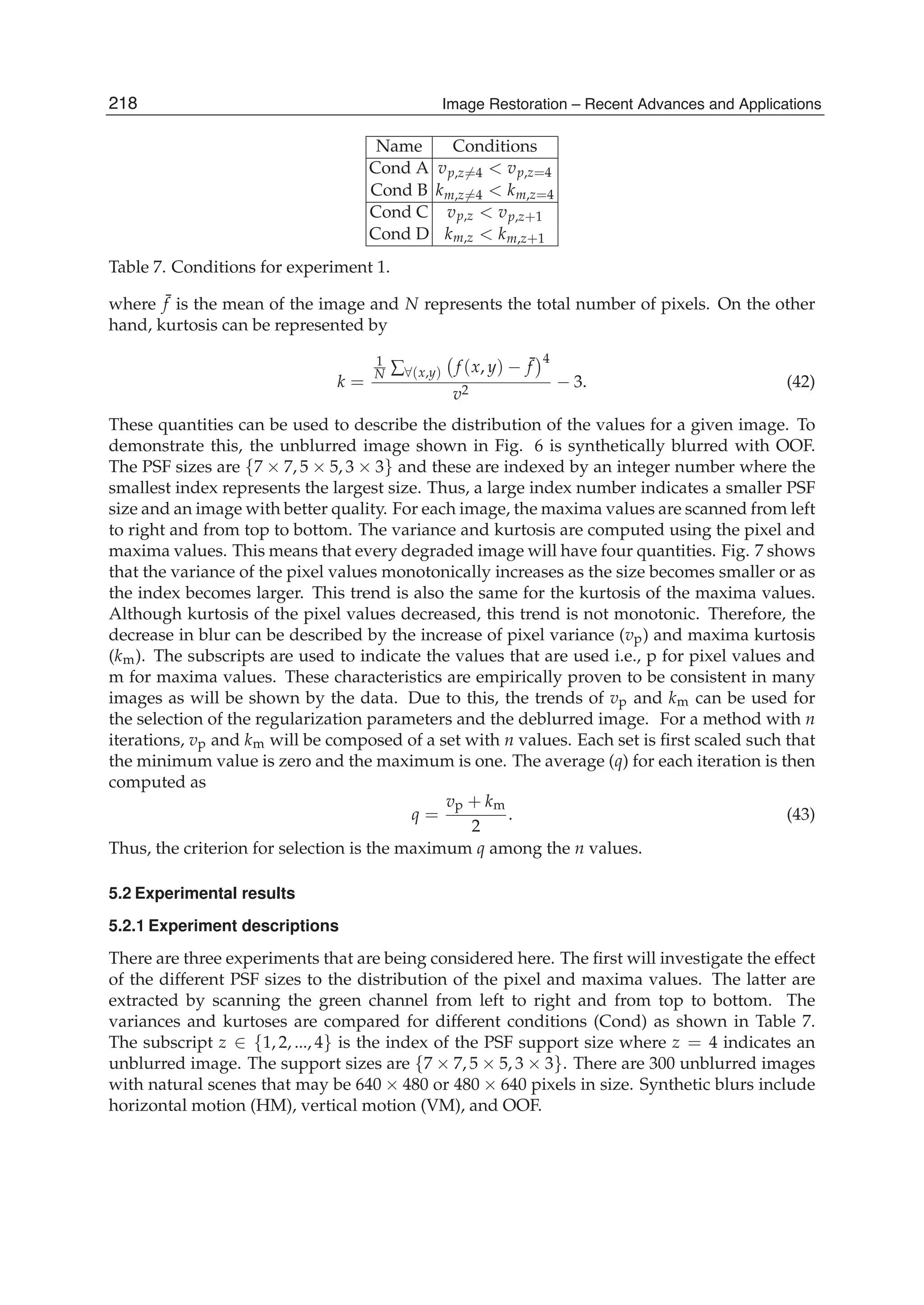
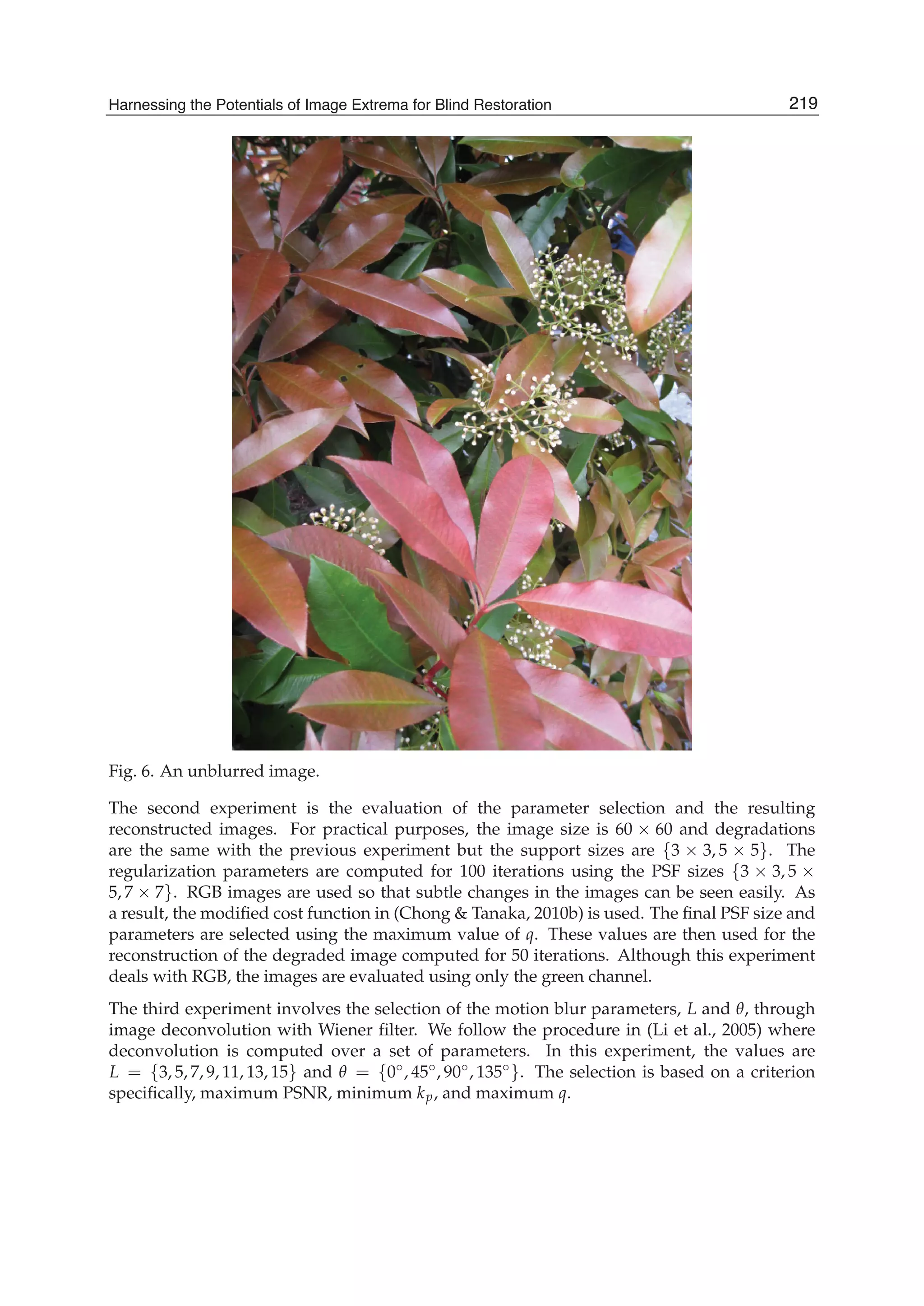
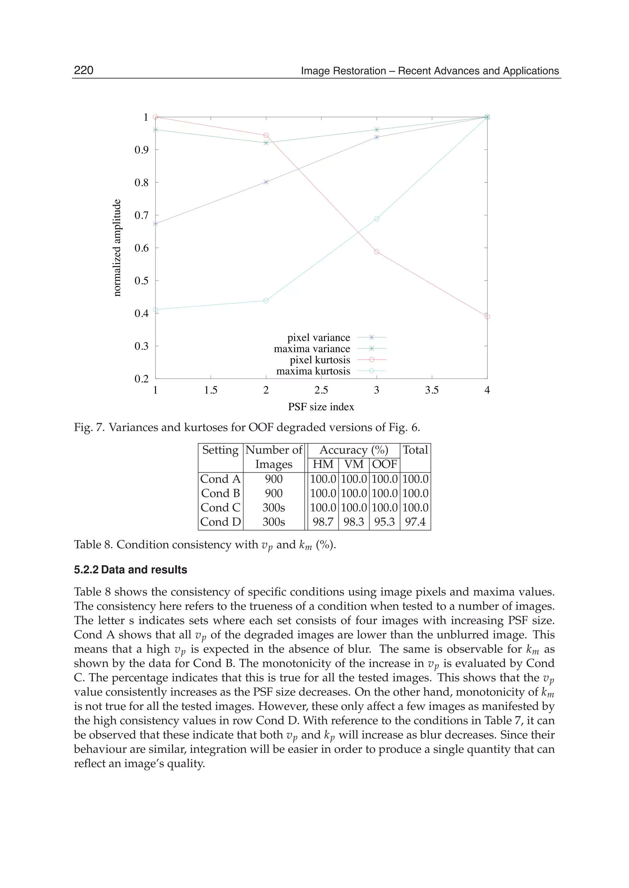
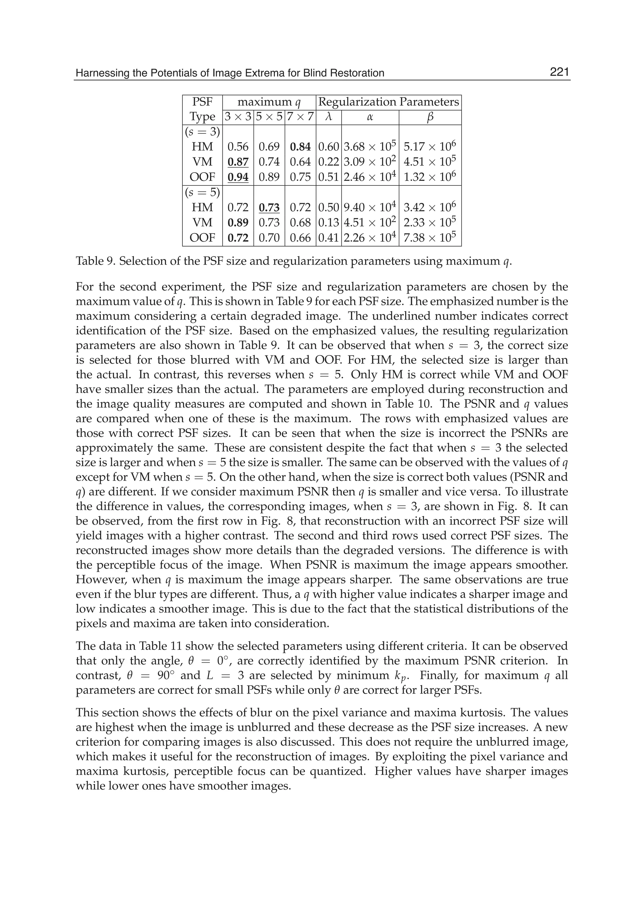
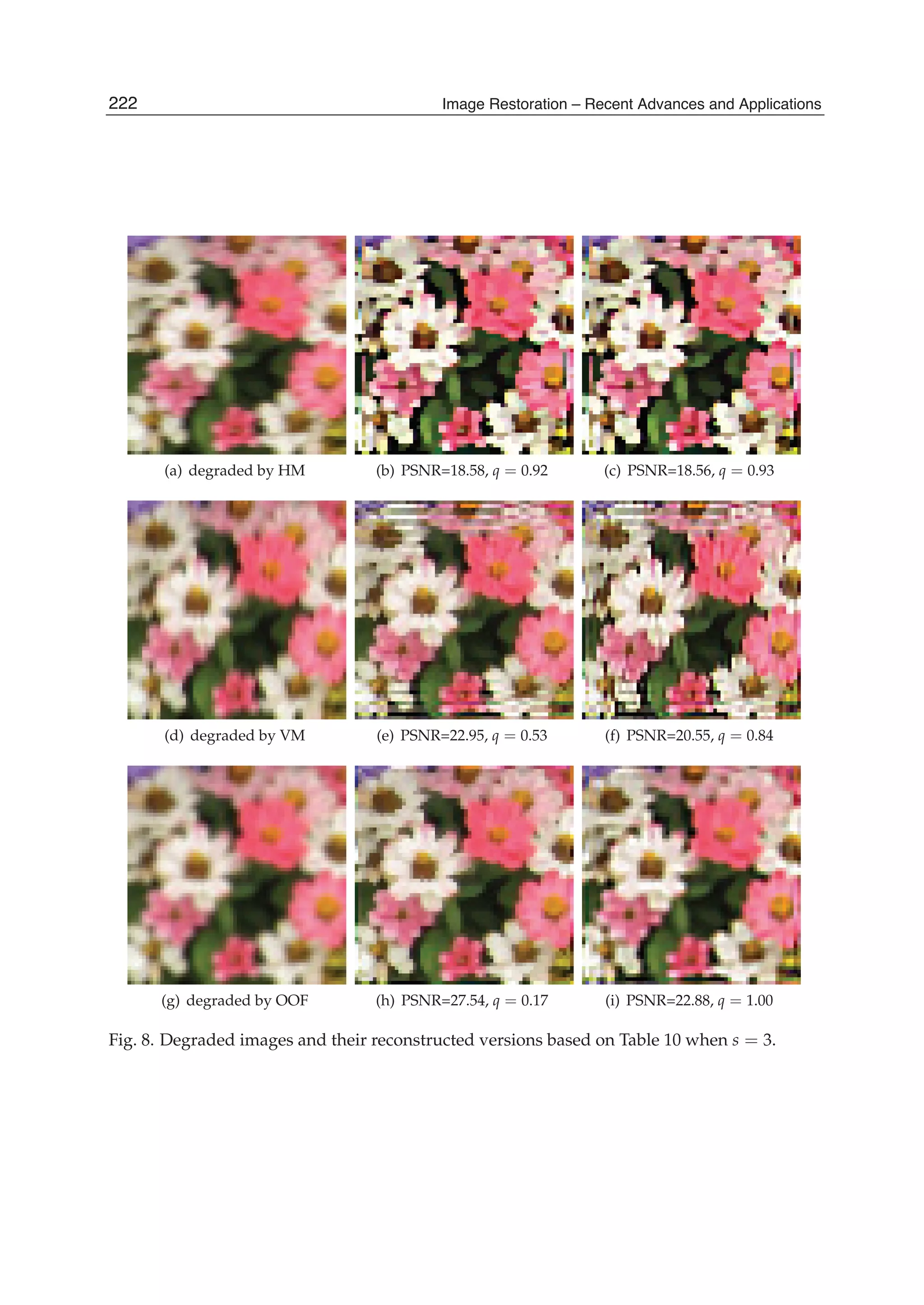
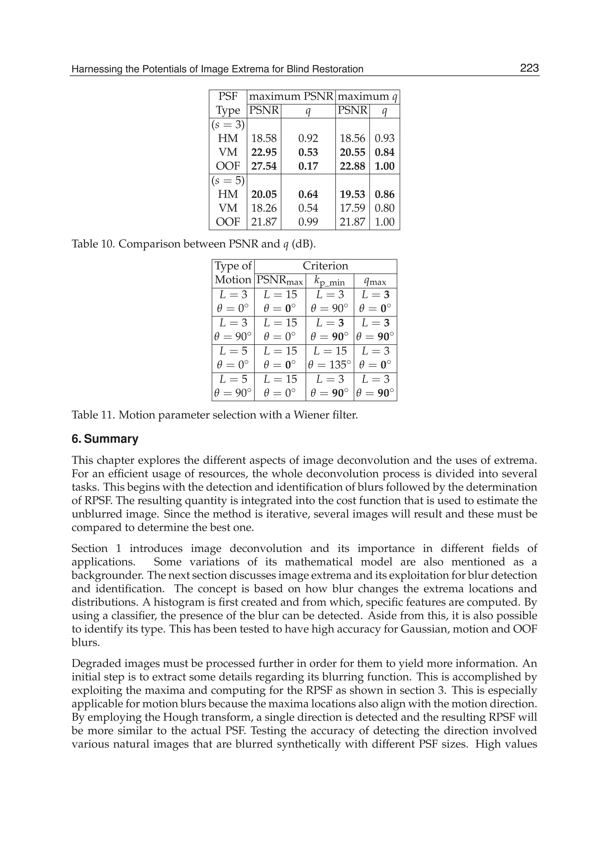


![11
Image Restoration for
Long-Wavelength Imaging Systems
Min-Cheng Pan
Department of Electronic Engineering, Tungnan University
New Taipei City
Taiwan
1. Introduction
1.1 Overview
Basically, the quality of an image can be evaluated on its spatial and spatial-frequency
resolutions, image interpolation and superresolution are perhaps the way to respectively
produce high spatial and spatial-frequency resolutions of images especially for a single down-
sampled image. For convenience, the term “hyper-resolution” used here represents the
approach to enhancing both the spatial and the spatial-frequency resolutions of an image.
As known, the process of decimation or down-sampling is an effective way often used to
reduce image sizes, thus, reducing the amount of information transmitted through the
communication channels and the local storage requirements, while trying to preserve as
much as possible the image quality. Conversely, the reverse procedure of this, referred to as
interpolation or up-sampling, is useful in restoring the original high resolution image from
its decimated version or for resizing or zooming a digital image. Decimation and
interpolation are used for several purposes in many practical applications, such as
progressive image transmission systems, multimedia applications, and so forth. A number
of conventional interpolation techniques [Hou & Andrews, 1978; Jain, 1989; Keys, 1981] have
been proposed to increase the spatial resolution of an image. Undoubtedly, these techniques
degrade the quality of the magnified image.
Furthermore, images may be corrupted by degradation such as blurring distortion, noise, and
blocking artifacts. These sources of degradation may arise during image capture or processing
and have a direct bearing on visual quality. Various methods of restoration have been
described in the literature; this diversity reveals the importance of the problem and its great
difficulty. The purpose of image deconvolution or restoration is to recover degraded images
by removing noise, highlighting image contrast, and preserving edge features of image.
Image superresolution was developed in 1950s to improve image quality and pilot research
of this field is derived from the early work (Toraldo di Francia, 1952, 1955) where the term
“superresolution” was used in the paper. Following that, clear definition, description and
some of the obvious contribution to this field can be found in the work (Gerchberg, 1974;
Hunt & Sementilli, 1992) in which their work, superresolution, was meant to seek to recover](https://image.slidesharecdn.com/imagerestorationrecentadvancesandapplications-160714160024/75/Image-restoration-recent_advances_and_applications-239-2048.jpg)
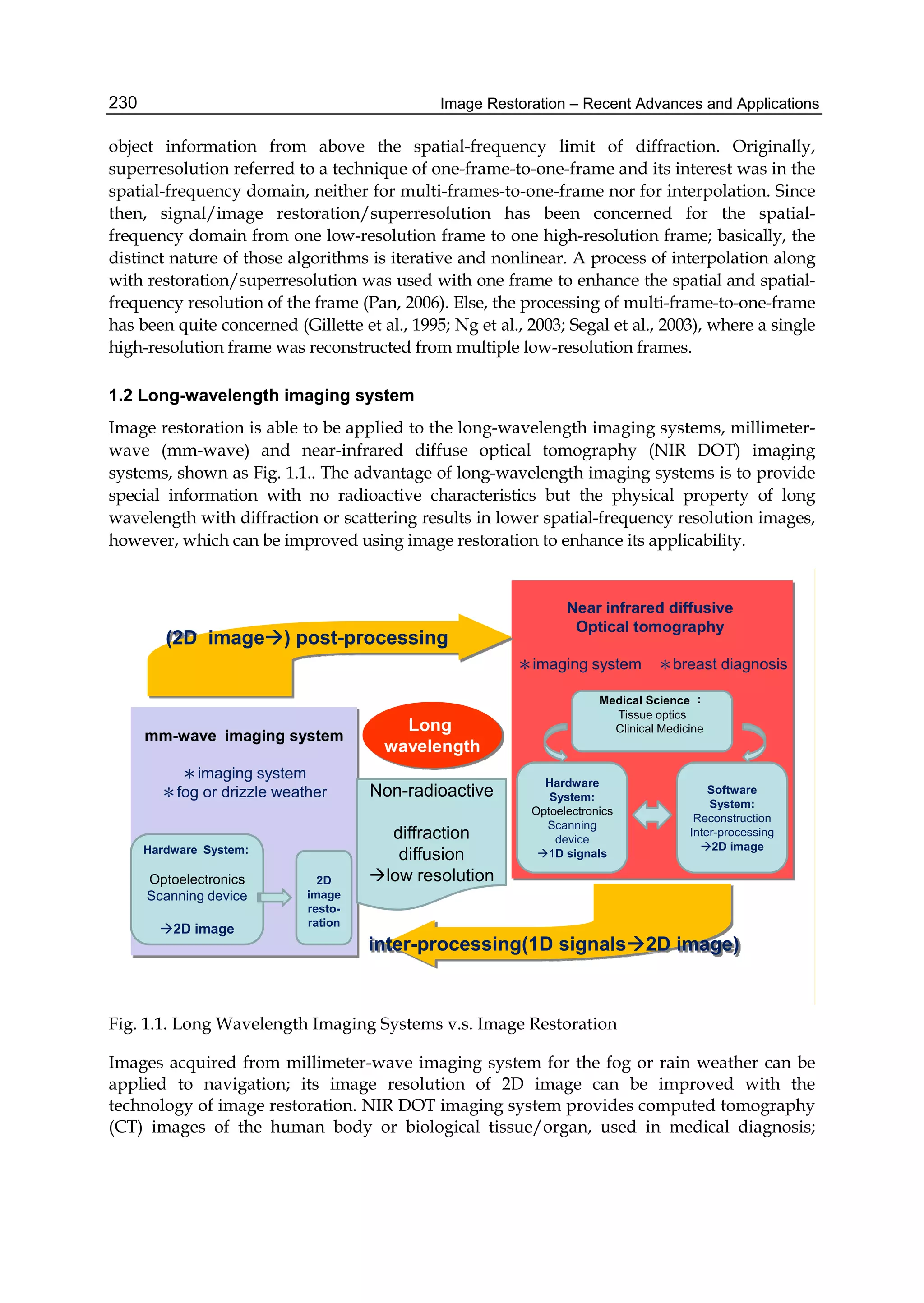
![Image Restoration for Long-Wavelength Imaging Systems 233
2.3 Forward problem & inverse problem
In a common imaging system, the image is formed as the above description in which finding
an estimated original signal/image (f) is an inverse problem for a given corrupted
signal/image (g) while the reverse process is a forward problem. In tomographic imaging, the
reconstruction of optical-property images is done iteratively using a Newton method,
requiring inversion of a highly ill-posed and ill-conditioned matrix. The goal of DOT is to
estimate the distribution of the optical properties in tissue from non-invasive boundary
measurements. For the purpose of determining the optical properties (the absorption
coefficient and the diffusion/scattering coefficient) from measurement data, which is an
inverse problem in DOT, a forward model is needed to describe the physical relation between
the boundary measurements of tissue and the optical properties that characterize the tissue.
2.3.1 Forward problem in DOT
In general, such a forward model of NIR DOT that gives the description of this physical
relation is the diffusion equation,
, , ,a
i
S
c
r r r r r (2.2)
where , r is the photon density at position r and is the light modulation frequency.
,S r is the isotropic source term and c is the speed of light in tissue. a and denote
the optical absorption and diffusion coefficients, respectively. In addition, the finite element
method (FEM) and a Robin (type-III) [Brendel & Nielsen, 2009; Holboke et al., 2000]
boundary condition are applied on Eq. (2.2) to solve this forward problem, i.e., calculating
the photon density for a given set of optical property within the tissue.
2.3.2 Inverse problem in DOT
Owing to the non-linearity with respect to the optical properties, an analytic solution to the
inverse problem in DOT is absent. Instead, the numerical way of obtaining the inverse
solution is to iteratively minimize the difference between the measured diffusion photon
density data, M
Φ , around the tissue and the calculated model data, C
Φ , from solving the
forward problem with the current estimated optical properties. This data-model misfit
difference is typically defined as follows,
22
1
MN
C M
i i
i
(2.3)
where MN is the number of measurements.
By means of the first order Taylor series to expand Φ , one can get Eq. (2.4),
,
C C
M C
a
a
Φ Φ
Φ Φ μ κ
μ κ
(2.4)](https://image.slidesharecdn.com/imagerestorationrecentadvancesandapplications-160714160024/75/Image-restoration-recent_advances_and_applications-243-2048.jpg)
![Image Restoration for Long-Wavelength Imaging Systems 235
p.s.f., and a user-defined weight (α). Ψ can have various forms derived from the different
algorithms. As known, there are several approaches to enhancing image quality including
non-iterative restoration algorithms such as a Gaussian filter and non-linear iterative
algorithms such as Poisson maximum a posteriori superresolution algorithm.
3.1 Non-iterative methods
Non-iterative restoration algorithms are described in this sub-section such as the inverse
and Wiener filters usually recovering the spatial-frequencies below the diffraction limit.
Filters in the Fourier domain are respectively given by the following expressions:
Inverse Filter =
1
H
(3.4)
However, Eq. (3.4) is not able to be directly implemented; usually, one uses a so called
pseudo-inverse filter with a small constant ε as below.
Pseudo-inverse Filter =
1
H
(3.5)
Wiener filter is described as Eq. (3.6) in the following.
Wiener Filter =
2
n f
*
[ / ]
H
H
(3.6)
where H is the modulation transfer function (MTF) of p.s.f.; the superscript asterisk (*)
denotes the complex conjugate; [n/f], the ratio of noise-to-signal. n and f represent the
power spectral densities for noise and the true images, respectively. Apparently, applying
the Wiener filter to the restoration problem has to know the power spectral densities for the
noise and the original image (or more precisely, their ratio). Unfortunately, this a priori
knowledge is not available in most cases. Nevertheless, the noise-to-signal ratio (NSR),
[n/f], is usually approximated by a small constant ε. In such a case, the Wiener filter
becomes
2
*H
H
(3.7)
Wiener filtering achieves a compromise between the improvement obtained by boosting the
amplitude of spatial-frequency coefficients up to the diffraction limit and the degradation
that occurs because of the noise amplification of the inverse filtering. Noise propagation
tends to be reduced by the convolution with p.s.f.; this has a smoothing effect in the result.
This fact reveals that Wiener filtering is more immune to noise than inverse filtering.
3.2 Iterative methods
3.2.1 Recursive wiener filter
This technique is briefly described here; further, a more detailed description of the im-
plementation of this algorithm can be found in the literature [Kundur & Hatzinakos, 1998].](https://image.slidesharecdn.com/imagerestorationrecentadvancesandapplications-160714160024/75/Image-restoration-recent_advances_and_applications-245-2048.jpg)
![Image Restoration for Long-Wavelength Imaging Systems 237
1
1
n
g
h
f h
C exp (3.12)
C can be regard as the correction term during the iterative restoration process. In terms of
the operation of the Poisson MAP, it is an iterative algorithm where successive estimate of
the restored image is obtained by multiplication of the current estimate by a quantity close
to one. The quantity close to one is a function of the detected image divided by a
convolution of the current estimate with p.s.f.. Indeed, one can replace the exponential in
Eq. (3.12) by the first order approximation ex ~ 1+x because of low contrast in a blurred
signal/image to achieve Eq. (3.13).
1
~ 1 1
n
g
h
f h
C (3.13)
Thus, Eq. (3.11) can approach to Eq. (3.14).
1 1 1
1
~ 1n n n n n
n
g
f f h f f
f h
f (3.14)
Equation (3.14) shows that the Poisson MAP superresolution is consistent with Eq. (3.2).
Experience reveals that when implemented for simple point objects, the Poisson MAP
algorithm is able to expand the bandwidth much more than done for more complex objects
and the Poisson MAP superresolution algorithm requires hundreds of iterations for a final
solution.
3.3.2 Improved P-MAP
Following that, the Poisson MAP can be improved by itself by operating upon the edge map
with a re-blurring technique; that is, the g and fn-1 of the Poisson MAP are replaced by the
corresponding gradients of the g ⊗ h and fn-1 along with the integrated p.s.f. (h ⊗ h).
Mathematically, it is shown that
1
1
( )'
( )' ( 1 ( )
( )' ( )
n n
n
g h
f f h h
f h h
)'exp (3.15)
Thus, the final hyper-resolved image f can be obtained by integrating (fn)’. The whole
process of this improved Poisson MAP includes re-blurring, differentiation, restoration,
integration, and then correction for a DC offset. More details concerning this algorithm can
be found in the author’s previous work [Pan, 2003].
3.4 Regularization
Regularization presents a very general methodology for image restoration. The main
technique of a regularization procedure is to transform this ill-posed problem into a well-
posed one. Roughly speaking, restoration problem with regularization comes down to the
minimization problem [Chen et al., 2000; Landi, 2007].](https://image.slidesharecdn.com/imagerestorationrecentadvancesandapplications-160714160024/75/Image-restoration-recent_advances_and_applications-247-2048.jpg)
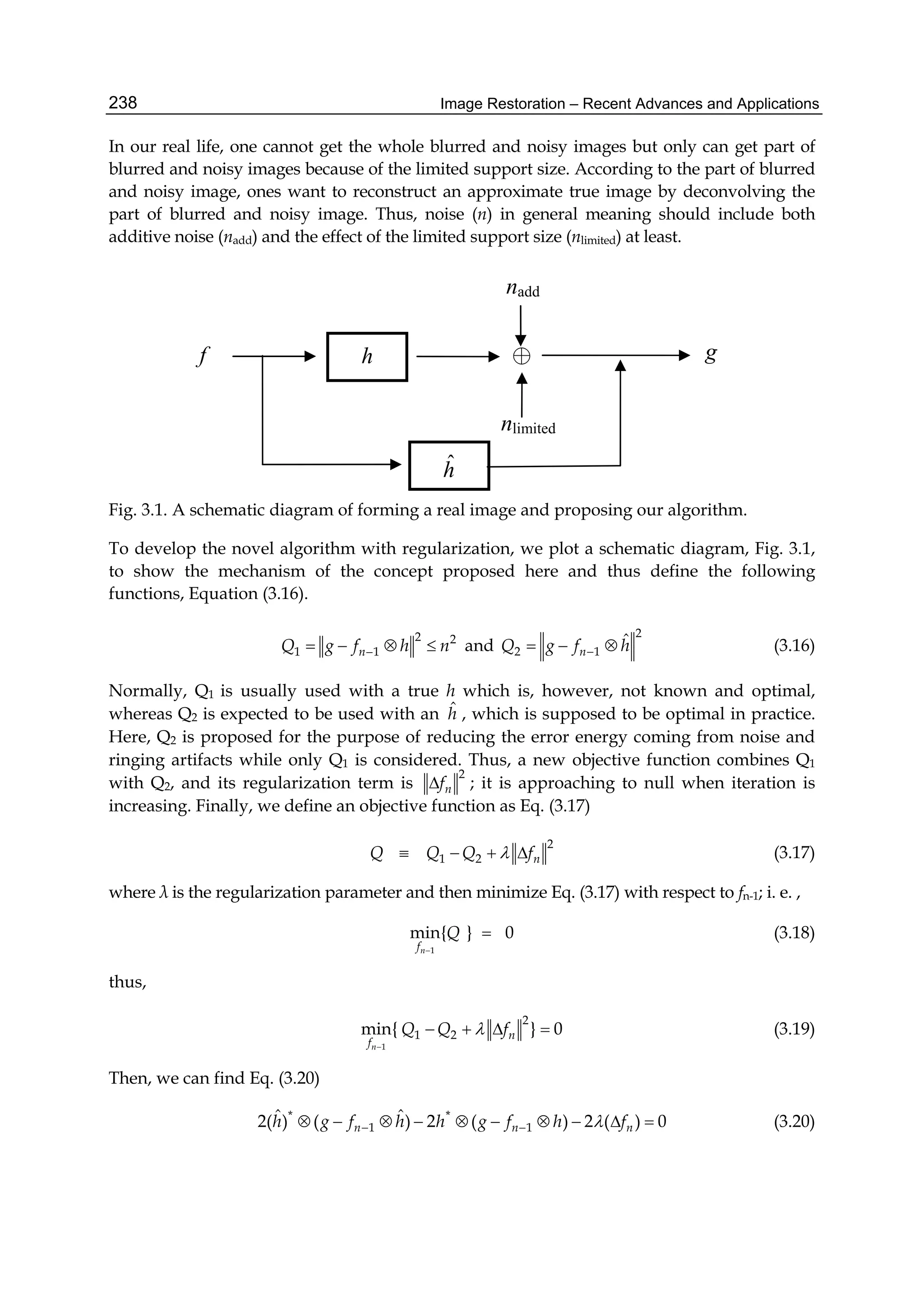
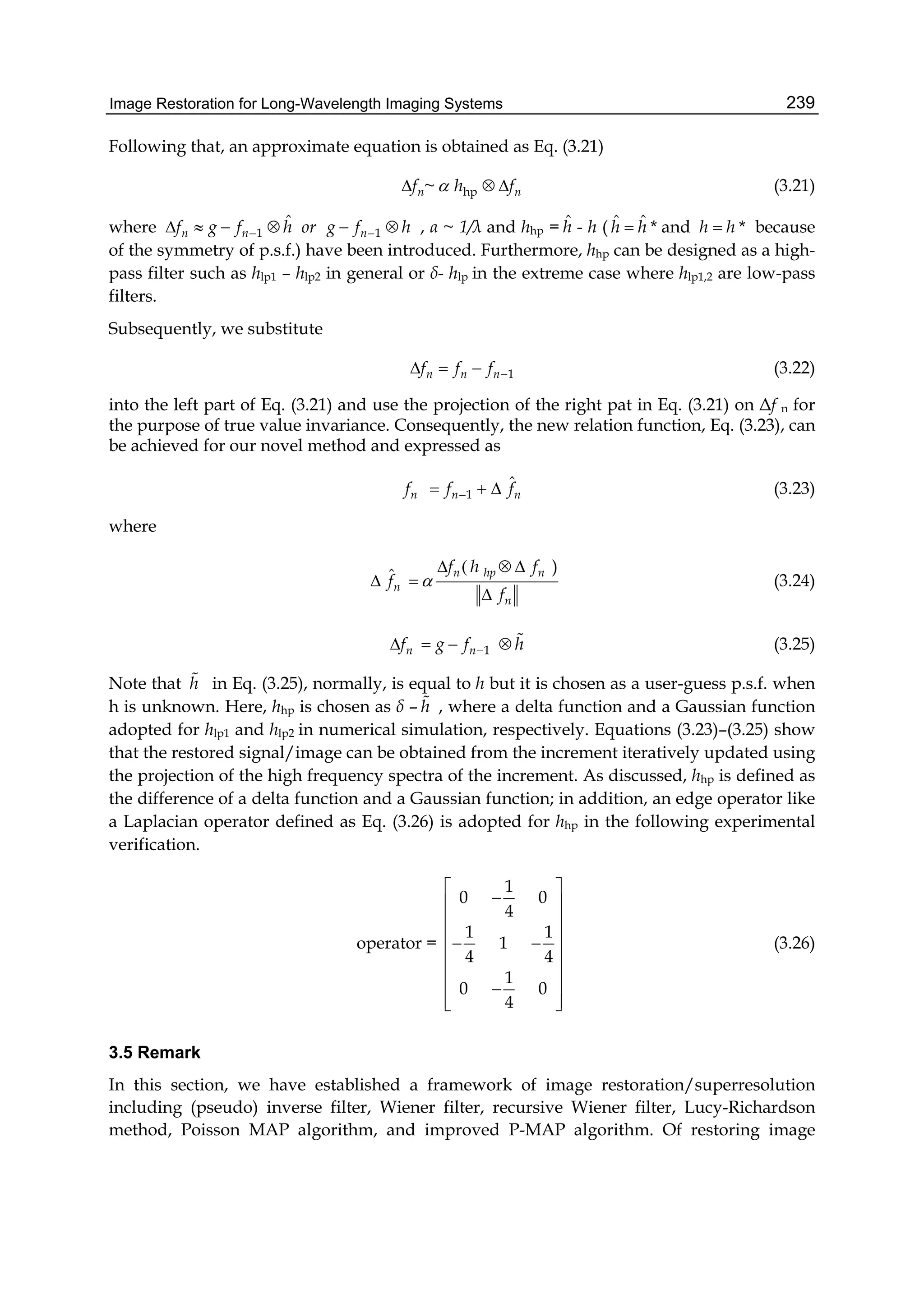
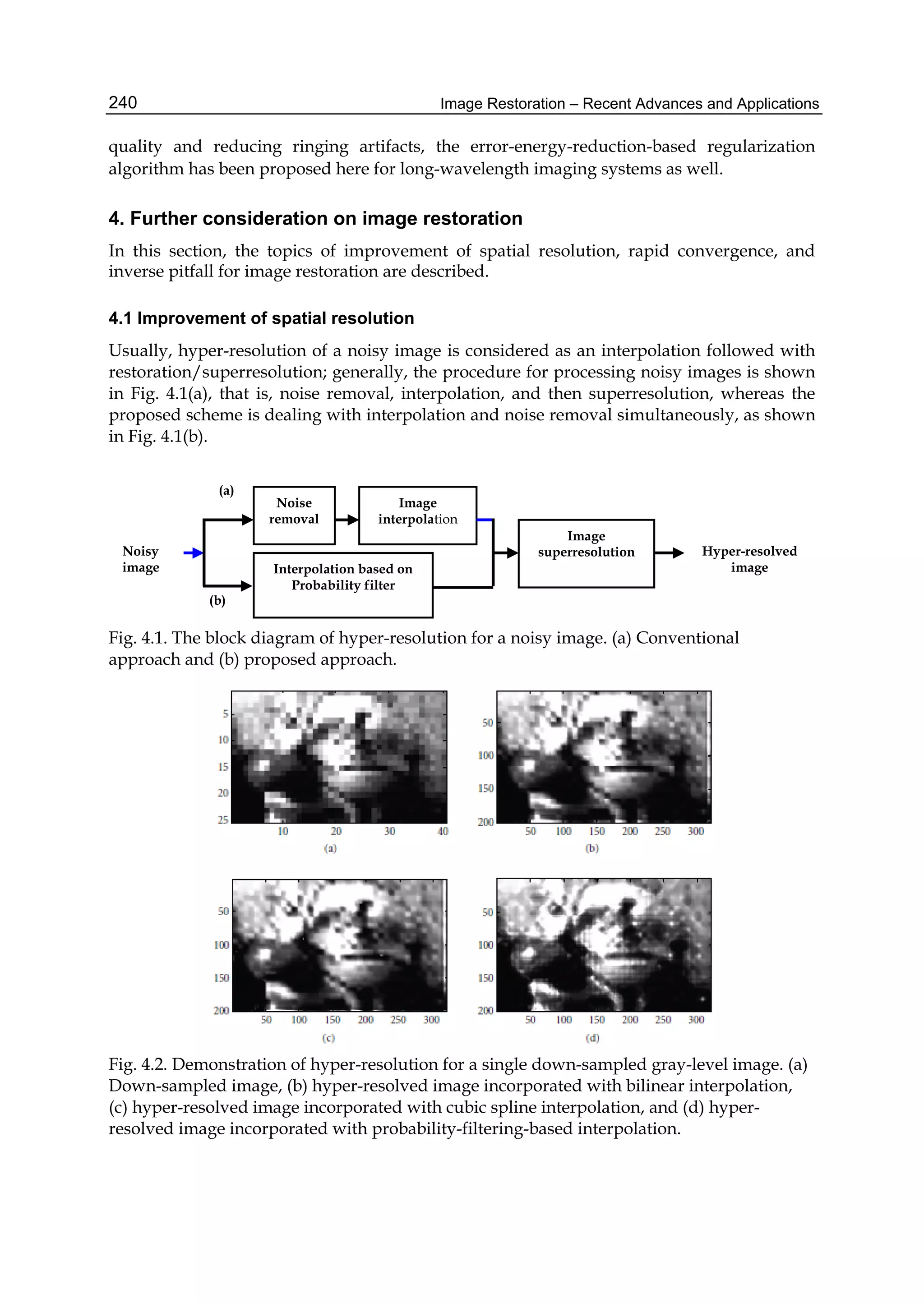
![Image Restoration for Long-Wavelength Imaging Systems 241
In this section, we address an approach to simultaneous image interpolation and smoothing
by exploiting the probability filter [Pan & Lettington, 1998] coupled with a pyramidal
decomposition, thereby extending the conventional applications of the probability filter
originally designed for noise removal. Then, the improved Poisson maximum a posteriori
(MAP) superresolution [Pan & Lettington, 1999; Pan, 2002] is performed to reconstruct the
high spatial-frequency spectrum of the interpolated image. Thus, the hybrid scheme shown
in Fig. 4.1(b) is proposed for enhancing the spatial and the spatial-frequency resolutions of a
down-sampled image. For more detailed description and examples, readers can refer to the
previous work [Pan, 2006]. To illustrate the performance of this proposed scheme,
comparisons are shown among the superresolution coupled with different interpolators as
the following examples, Fig. 4.2 and Fig. 4.3.
Fig. 4.3. Demonstration of hyper-resolution for a single down-sampled noisy gray-level
image. (a) Down-sampled image, (b) hyperresolved image incorporated with bilinear
interpolation, (c) hyper-resolved image incorporated with cubic spline interpolation, and (d)
hyper-resolved image incorporated with probability-filtering-based interpolation.
4.2 Rapid convergence
As known, restoration/superresolution or the reconstruction of optical-property images
with an iteration procedure is usually computed off-line and computationally expensive.
Most of studies, however, focused mainly on improving the spatial and spatial-frequency
resolutions. If a real-time resolution processing is required, dedicated reconstruction
hardwares or specialized computers are mandatory. Moreover, fast reconstruction
algorithms should also be considered to reduce the computation load. It is worth
emphasizing that our proposed method can reduce computation time with the
regularization term which is designed on the viewpoint of the update characteristics in the
iteration procedure but not utilizing any spatial/spectral a priori knowledge or constraints;
some results can be found in the author’s work [M.-Cheng & M.-Chun Pan, 2010]. Here, we](https://image.slidesharecdn.com/imagerestorationrecentadvancesandapplications-160714160024/75/Image-restoration-recent_advances_and_applications-251-2048.jpg)
![Image Restoration – Recent Advances and Applications242
show how to speed up the computation to find an inverse solution for reconstructing
optical-property images by using regularization with an iteration domain technique;
similarly, this proposed method is capable of being applied to image
restoration/superresolution for other imaging systems.
4.2.1 Algorithm of rapid convergence
Image reconstruction tasks contain forward modeling and inverse problem. The forward
computation consists in obtaining the intensity out of a subject under investigation for a
given source, and the initial-guess (or iterated result) on scattering and absorption
coefficients. The inverse computation is to compute the scattering and absorption
coefficients for a known light source and measured intensities in an iterative manner.
Since we utilize cw light illumination or DC data, the physical process of NIR light
illuminating through a highly-scattering medium can be approximated by the steady-state
diffusion equation
( ) ( ) ( ) ( ) ( ) r r r r raD S , (4.1)
where ( )S r and ( ) r denote the source and the intensity, respectively, as well as ( )a r , c
and ( )rD are the absorption coefficient and the diffusion coefficient, respectively. For
solving Eq. (4.1), the boundary condition, ˆ D n Flux , and finite element method
are employed. Thus, the following discrete equations can be obtained [Paulsen and Jiang,
1995]
A C , (4.2)
where A and C are matrices dependent on the optical properties and the source-detection
locations, respectively. The forward solution, , can be explicitly evaluated by Eq. (4.2).
Partially differentiating Eq. (4.2) with D
and
, respectively, yields
' 1 ' 1 '
A A A C
. (4.3)
With an approximation to applying the Newton-Raphson method and ignoring higher order
terms, we obtain
J (4.4)
where the Jacobian matrix J denotes the matrix consisting of b
kD
and b
l
, is the vector
composed of Dk and l, and is the vector with differences between calculated
intensities (Φcal.) and measured intensities (Φmeas.). Also, Dk for k = 1, 2, …, K and μl for l = 1,
2, …, L are the reconstruction parameters for the optical-property profile. The optical-
property image reconstruction is actually a process of successively updating the distribution
of optical coefficients so as to minimize the difference between measured intensities and
computed ones from the forward process. More details can be found in [Paulsen and Jiang,
1995] where the Levenberg-Marquardt procedure was adopted to update the diffusion and
absorption coefficients iteratively.](https://image.slidesharecdn.com/imagerestorationrecentadvancesandapplications-160714160024/75/Image-restoration-recent_advances_and_applications-252-2048.jpg)
![Image Restoration for Long-Wavelength Imaging Systems 243
It is known that to solve Eq. (4.4) is an ill-posed problem. Tikhonov regularization is a
method stabilizing the inverse problem through incorporating a priori assumptions to
constraint the desired solution. It is able to convert an ill-posed problem into a well-posed
one, and further to improve an ill-conditioned problem. The regularization term (penalty
term) introduced in the process regularizes the problem and makes the update stable. It also
strengthens the robustness of algorithm to noisy data with the adequate design of the
regularization term. Generally, Tikhonov regularization is to optimize this ill-conditioned
problem as
2
min J
subject to ( ) E (4.5)
where () is a constraint on the estimate , and E is a quantity confining the constraint
to be an energy bound. Applying Lagrange optimization technique, we seek a solution to
the constrained objective function
2
J (4.6)
with the condition
2
min min J
, (4.7)
where λ is referred to as the regularization parameter. A solution to Eq. (4.7) is given by
2 ( ) 0T
J J
, (4.8)
and equivalently
( )
2
T T
J J J
(4.9)
where Eq. (4.9) is a constrained estimate of , but becomes an unconstrained one when λ
equals to zero. It is noted that the minus sign in Eq. (4.6), the objective function, corresponds
to the regularization term proposed here as the term is constrained to an energy bound.
4.2.2 Constraints on the spatial domain
A constraint on the spatial domain can generally be expressed as
2
( ) L (4.10)
where L can be the identity matrix (I) or the discrete Laplacian matrix [Pogue et al., 1999;
Davis et al., 2007].
If L is the identity matrix (I), a solution to Eq. (4.9) is given by
1
( - )T T
J J I J
. (4.11)](https://image.slidesharecdn.com/imagerestorationrecentadvancesandapplications-160714160024/75/Image-restoration-recent_advances_and_applications-253-2048.jpg)
![Image Restoration – Recent Advances and Applications244
On the other hand, if L is the discrete Laplacian matrix, substituting Eq. (4.10) into Eq. (4.9),
the corresponding solution is
1
( - )T T T
J J L L J
. (4.12)
Equation (4.11) is usually a primary inverse solution to optical-property image
reconstruction, which is also Levenberg’s contribution to the inverse problem; and Eq. (4.12)
is a constrained inverse solution implemented to improve the quality of the reconstructed
NIR DOT images, which is identical to Marquardt’s work.
4.2.3 Constraints on the iteration domain
In NIR DOT, it is also crucial to accelerate the computation. But, up to now, speeding up the
computation in the iteration domain has not been explored yet. Here we consider this issue
through the use of a Lorentzian distributed function taking a natural logarithm computation
as a constraint, i.e.
2 2
1
/
( )
( )
K L
p p
n
, (4.13)
where p is the calculated nodes in the subject under investigation and γ is a user defined
positive parameter. As can be seen, 1
( ) ln( )
p
, , meets the requirement of Eq.
(4.5). Performing the differentiation indicated in Eq. (4.9), we can obtain the solution in an
iterative formality
1
2 2
1
( ) +
( ) n
T T
n
n
I
J J J
I
. (4.14)
For further inspection in Eqs. (4.13) and (4.14), as known, μa and D are generally searched in
a range of [10-3:10-1] mm-1and mm, respectively; and thus Δχ is much smaller than a unit. It
can be proven that even the use of the natural logarithm in the constraint Ψ(Δχ) still makes
it a positive and finite value. The other reason to use ln is because the regularization term in
Eq. (4.14) still remains in a form of the Lorentzian distributed function derived from the
constraint associated with the Lorentzian distributed function in Eq. (4.13).
The Lorentzian distributed function, as depicted in Fig. 4.4, is employed here owing to its
following two characteristics:
a. Lorentzian distributed function has a sharp peak with a long tail, describing the
histogram distribution of Δχ, many of Δχ (~0) at its peak and a small rest of Δχ
distributing along its long tail, and
b. its histogram distribution can be further tuned with the parameter (γ) as iteration
increasing. Related to the consideration in convergence, the updated quantity, Δχ,
decreases, ranging from the peak to the tail, as the iteration increases whereas it has a
smooth distribution in the beginning stage of iteration.](https://image.slidesharecdn.com/imagerestorationrecentadvancesandapplications-160714160024/75/Image-restoration-recent_advances_and_applications-254-2048.jpg)
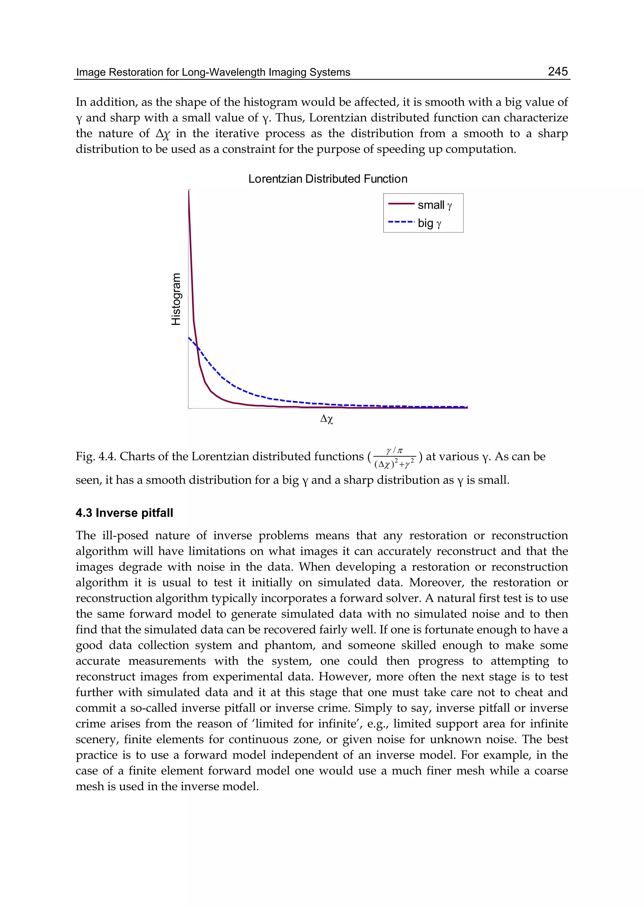
![Image Restoration – Recent Advances and Applications246
4.4 Remark
In this section, we have proposed some extra points about image restoration. Interpolator
with noise removal, design of regularization term for reducing computational burden, and
inverse pitfall/crime have been illustrated and discussed.
5. Related application
In this section, application to a mm-wave imaging system or near infrared diffuse optical
tomography using image restoration is demonstrated for post-processing or inter-
processing. To verify the proposed method in the previous section (Sec. 3.4), a computer-
generated signal/image and an image of real scene were tested.
5.1 Post-processing: Application to a millimeter-wave imaging system [Pan, 2010]
A 1-D noiseless signal and a 2-D noisy image were used, originally blurred with a p.s.f. of
Gaussian function plus additive white Gaussian noise. White Gaussian noise is defined with
a zero mean and variance, σ2, specified by a blurred signal-to-noise ratio (BSNR). Recall that
2
,
,
2
, 1
1010log
M N
i j
i j
f h f h
BSNR
MN
(in dB) (5.1)
where M, N are the dimension of the processed image and i, j are the indexes of a pixel and
X means the average value of X. In many practical situations, the blur is often unknown
and little information is available about the true image; therefore, several h
of the
Gaussian blur around the true σh were tested in the following examples; fo and α are chosen
to g and g , respectively. In this work, the stopping criterion is
0
nf
f
0.01% (for 1-D
signal) or 1% (for 2-D image). The mean square error (MSE) of the restored signal/image
relative to the original signal/image is provided here for the evaluation of image quality,
thus supporting the visual assessment.
The proposed algorithm was applied to a 1-D signal as well as both simulated and real
atmospherically degraded images, one of a simulated blur and one of a real blur. The
purpose of the simulation was to enable a comparative evaluation of the results given the
original signal/image and to explain the algorithm characteristics. In the real-blur example
shown here, a 256 × 400 pixel millimeter-wave image was tested and the image was
captured at 94 GHz by the Defence Evaluation and Research Agency, Malvern, UK.
For a comparison purpose, non-iterative Gaussian filtering was used in the case of 1-D
signal and the common Richardson–Lucy (RL) deconvolution method was implemented
using a built-in MATLAB function deconvlucy in the cases of both 1-D signal and 2-D
images. This RL method employs an iterative procedure to estimates the original
signal/image, and therefore requires an initial guess of it as well.](https://image.slidesharecdn.com/imagerestorationrecentadvancesandapplications-160714160024/75/Image-restoration-recent_advances_and_applications-256-2048.jpg)
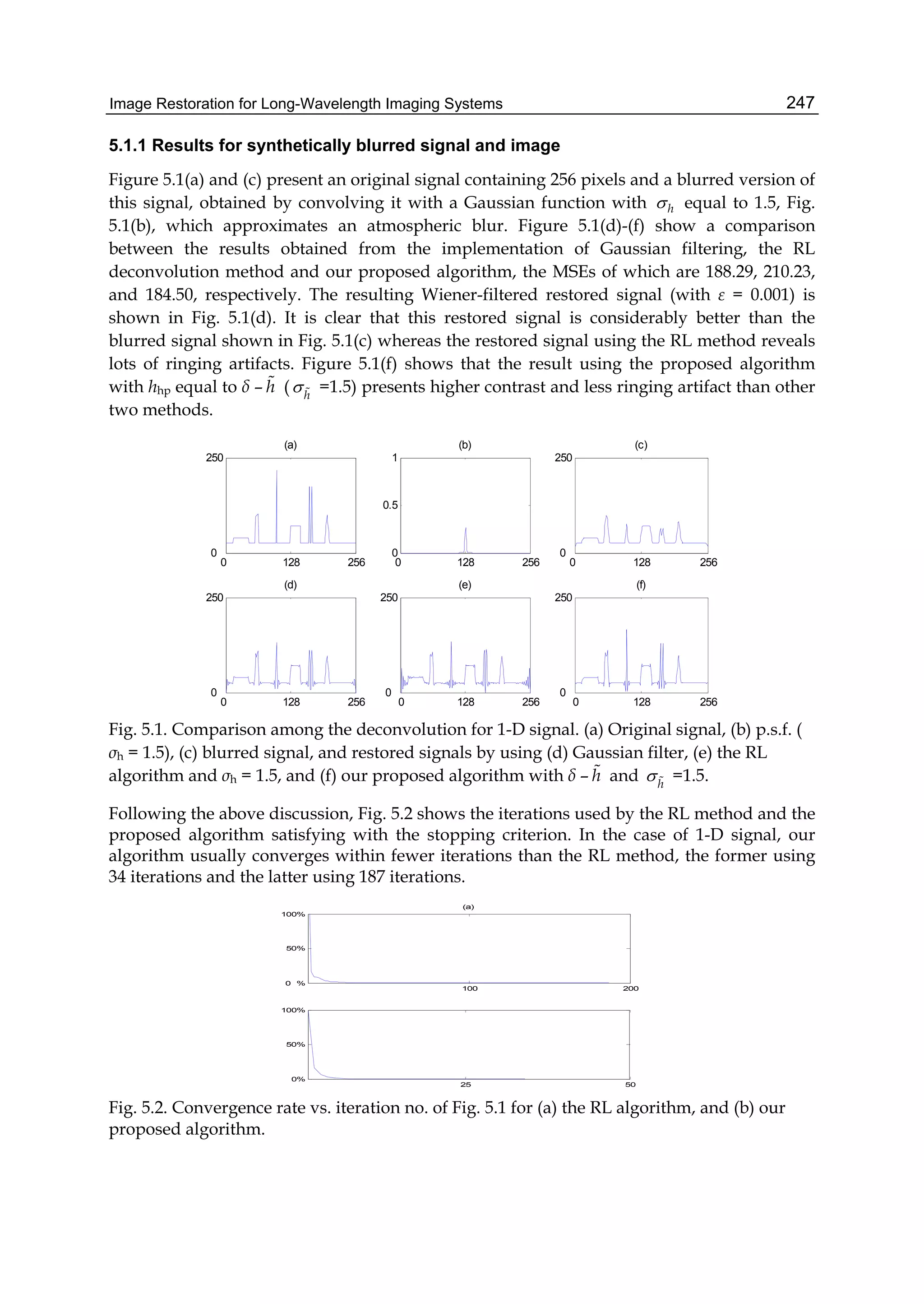
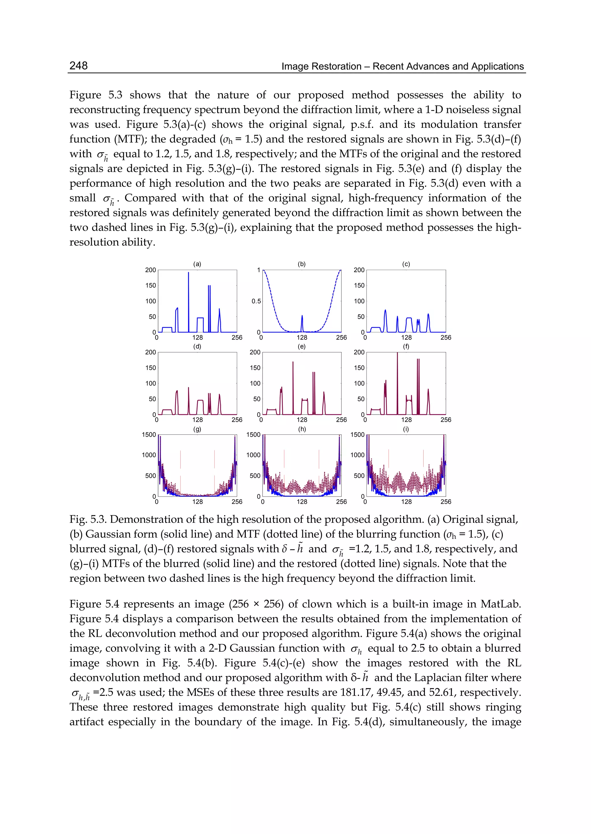
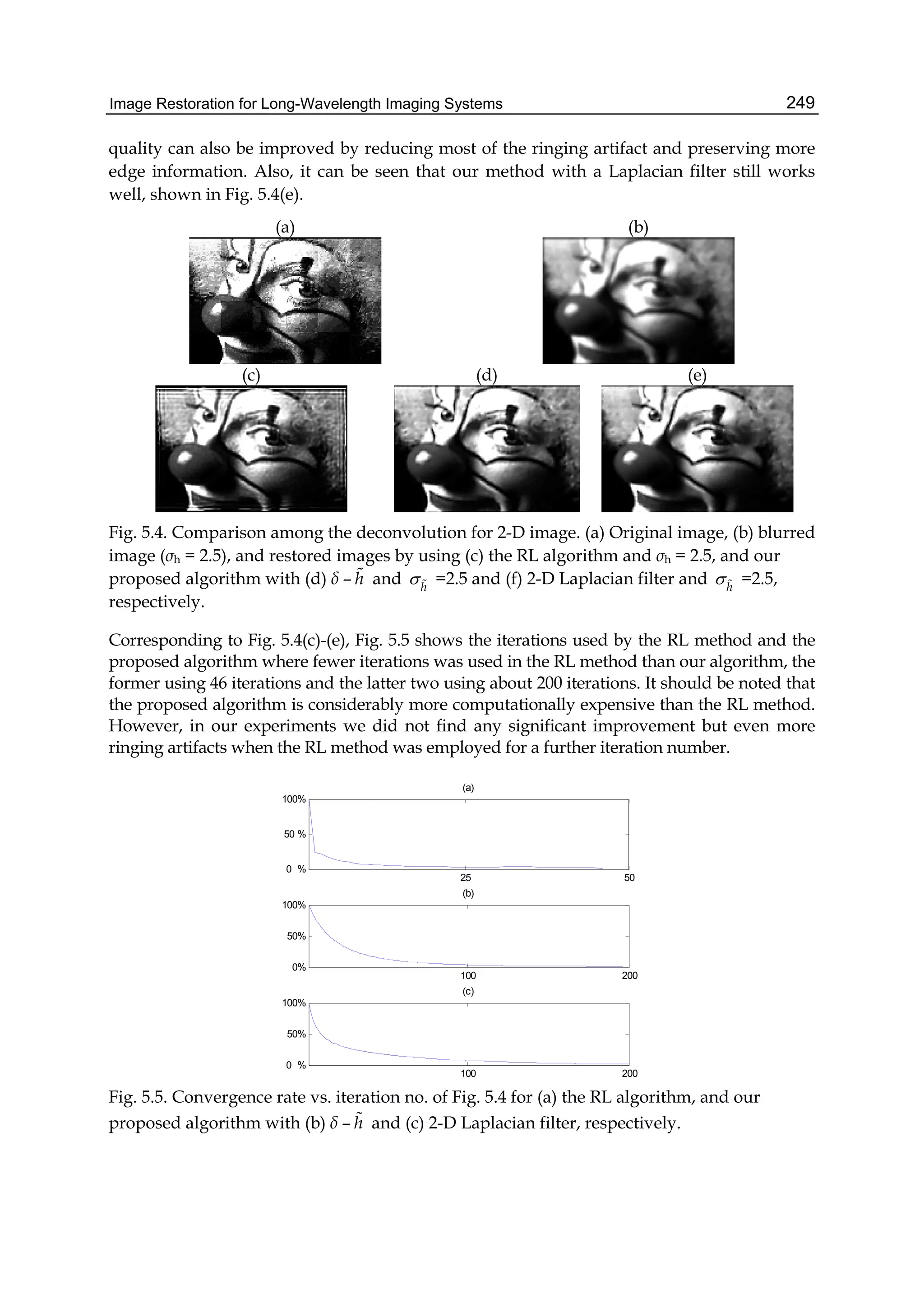
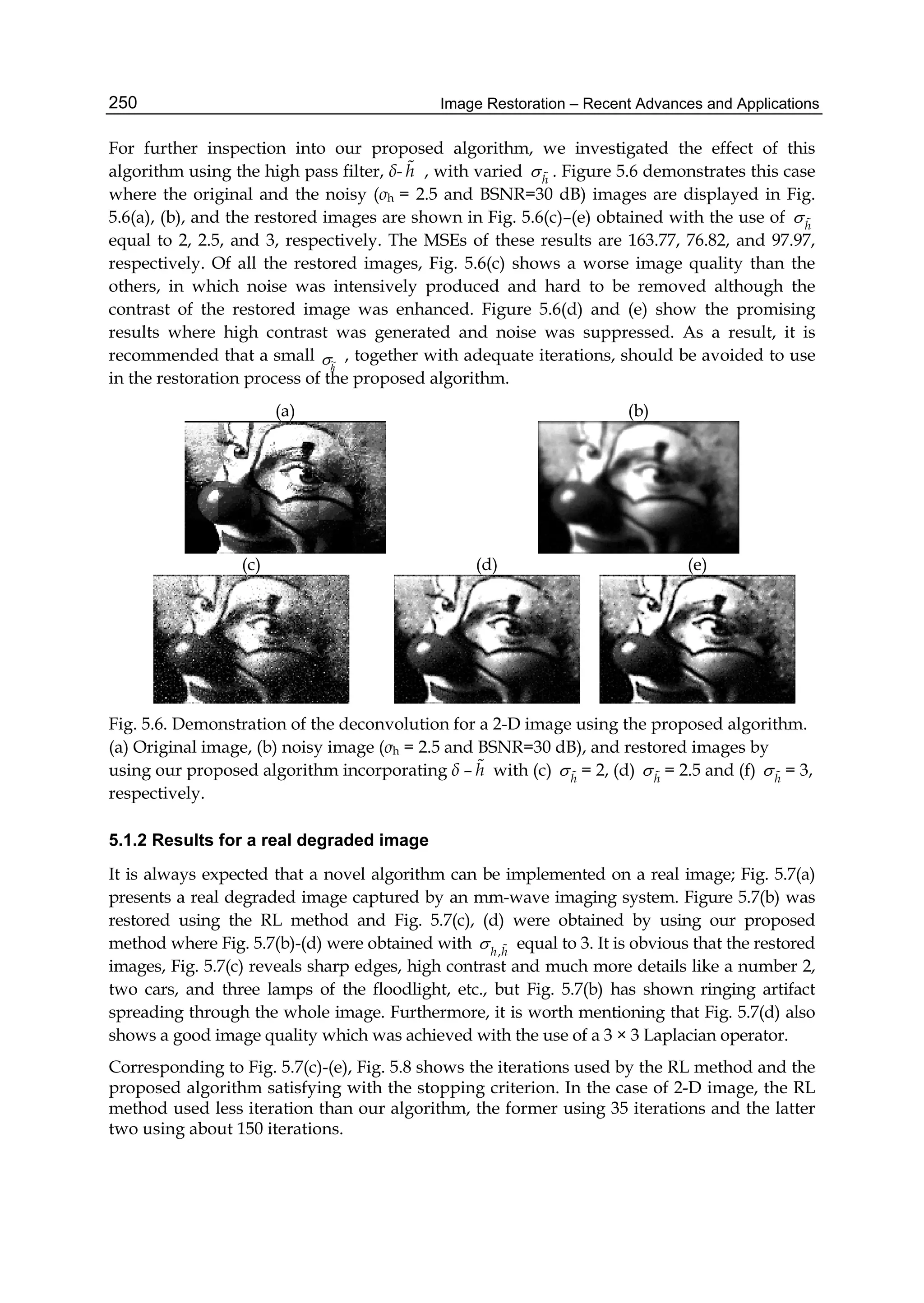
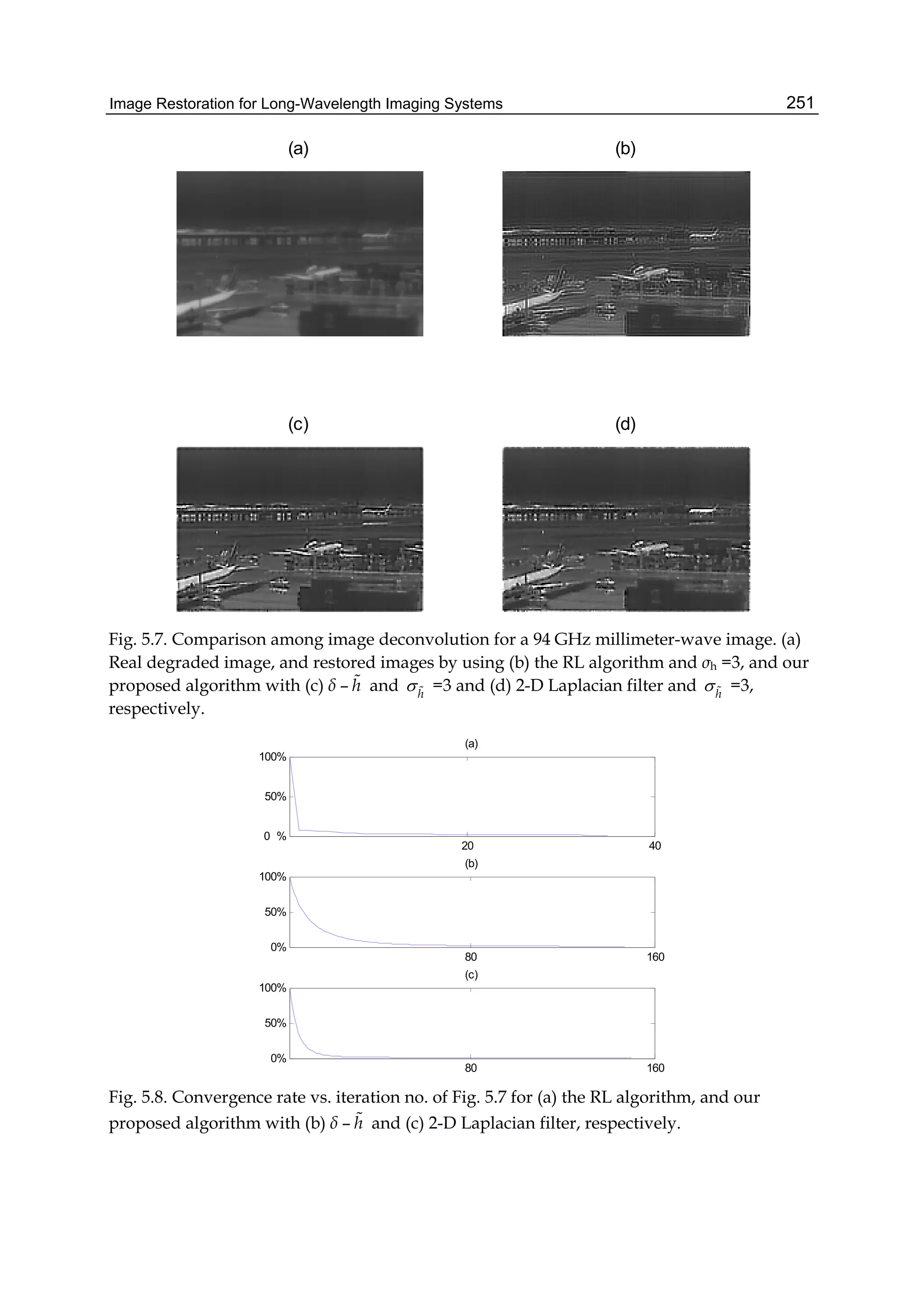
![Image Restoration – Recent Advances and Applications252
5.2 Inter-processing: Application to near infrared diffuse optical tomography
5.2.1 Rapid convergence algorithm applied to NIR DOT
Corresponding to Eq. (4.14), some parameters are chosen as
0.75max{ }T
J J , 0
2
( ) I , 2
2.5 n
n or e
, (5.2)
where the subscript n is the n-th iteration, “max” means the maximum value, and the
superscript T denotes a transposition operation. One way to improve the convergence rate is
using n as the Type-1 soft prior and using 2
2.5 n
n e
, an exponentially decreasing
form, as the Type-2 soft prior, where Type-1 is a parameter related to the system function
(Jacobian matrix) and Type-2 is a user-defined parameter. Both values of n have been
respectively employed to seek an inverse solution for comparison.
0
0.05
0.1
0 360
0
0.05
0.1
(g)
0
0.05
0.1
0 360
0
0.05
0.1
(h)
0
0.05
0.1
0 360
0
0.05
0.1
(i)
0 10 20 30
0
0.005
0.01
Convergence Rate
iteration no.
MSE(%)
0 10 20 30
0
0.005
0.01
Convergence Rate
iteration no.
MSE(%)
0 10 20 30
0
0.005
0.01
Convergence Rate
iteration no.
MSE(%)
0
0.05
0.1
0 360
0
0.05
0.1
(j)
0
0.05
0.1
0 360
0
0.05
0.1
(k)
0
0.05
0.1
0 360
0
0.05
0.1
(l)
2 incls.
3 incls.
2 incls.
3 incls.
2 incls.
3 incls.
(a) (b) (c)
(d) (e) (f)
(o)(n)(m)
Fig. 5.9. Reconstruction data through various priors with intensity signals corrupted by
Gaussian white noise (SNR=20 dB). Left column: constrained inverse solution with soft prior
1; middle column: constrained inverse solution with soft prior 2; right column: constrained
inverse solution with hard prior.
Figure 5.9 illustrates the comparisons between constrained solutions using soft priors (Type
1 and 2) and a hard prior, where the left, middle and right columns are the constrained
inverse solutions with soft prior 1, soft prior 2, and hard prior [M.-Cheng & M.-Chun Pan,
2010], respectively. Figure 5.9 (a-f) shows the 2D reconstructions of phantoms with two and
three inclusions, where slight discrepancy can be observed. Figure 5.9 (g-l) depicts their](https://image.slidesharecdn.com/imagerestorationrecentadvancesandapplications-160714160024/75/Image-restoration-recent_advances_and_applications-262-2048.jpg)
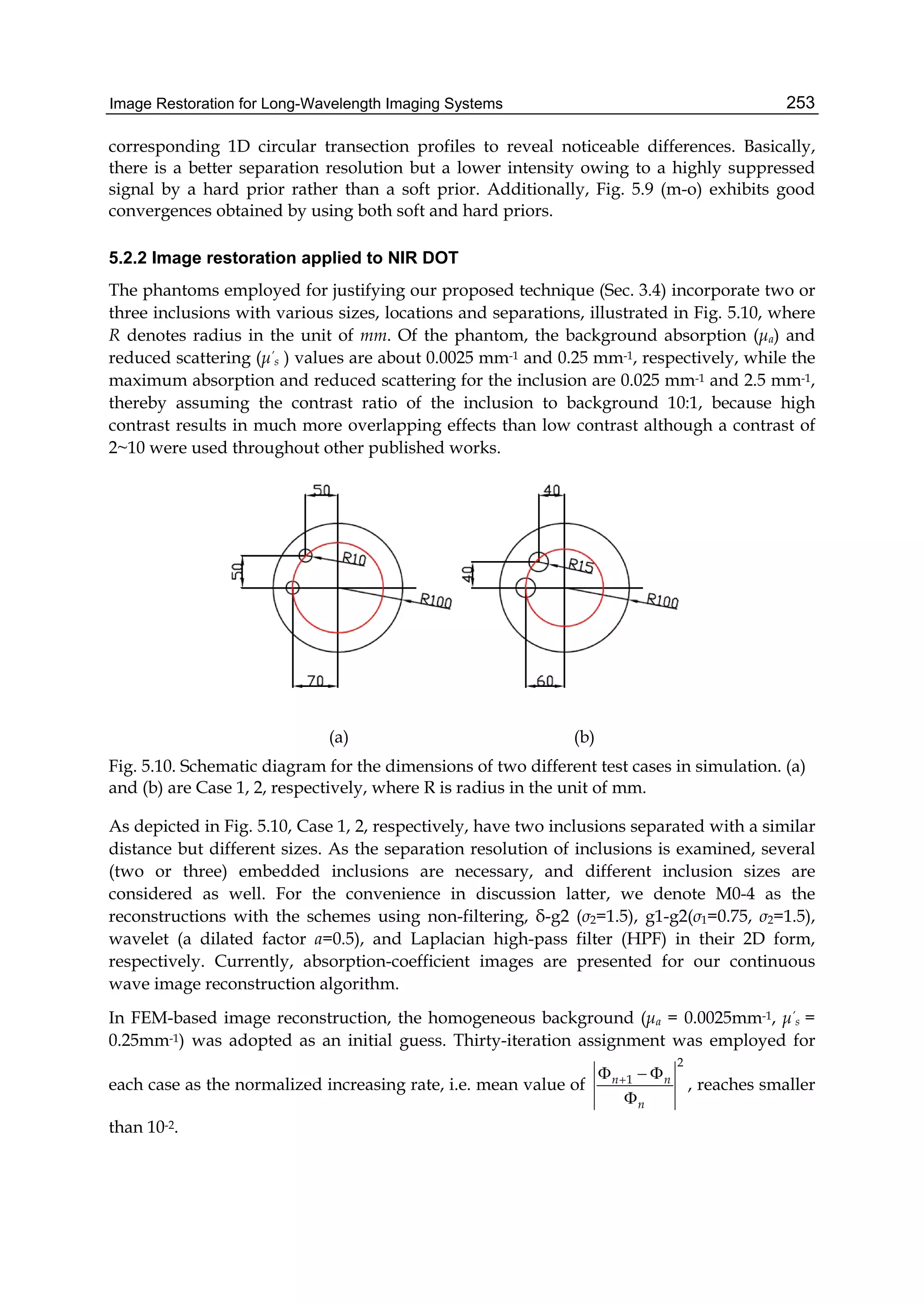
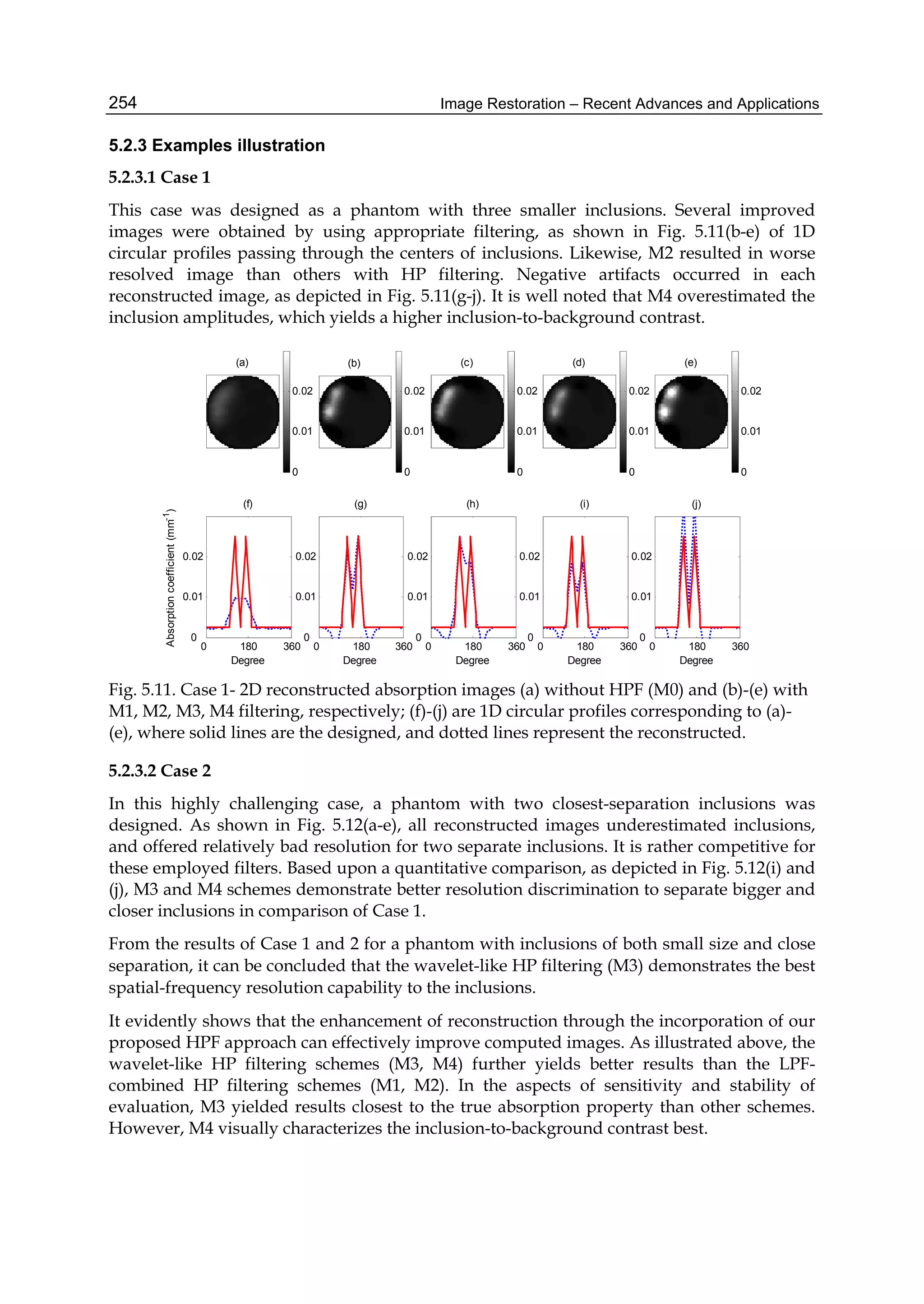
![Image Restoration for Long-Wavelength Imaging Systems 255
0 180 360
0
0.01
0.02
(f)
Degree
Absorptioncoefficient(mm-1
)
(b)
0
0.01
0.02
0 180 360
0
0.01
0.02
(g)
Degree
(c)
0
0.01
0.02
0 180 360
0
0.01
0.02
(h)
Degree
(d)
0
0.01
0.02
0 180 360
0
0.01
0.02
(i)
Degree
(a)
0
0.01
0.02
(e)
0
0.01
0.02
0 180 360
0
0.01
0.02
(j)
Degree
Fig. 5.12. Case 2- 2D reconstructed absorption images (a) without HPF (M0) and (b)-(e) with
M1, M2, M3, M4 filtering, respectively; (f)-(j) are 1D circular profiles corresponding to (a)-
(e), where solid lines are the designed, and dotted lines represent the reconstructed.
5.2.4 Performance investigation
In terms of the optical properties within the inclusion and background, it is worth noted that
the image reconstruction is not only pursuing qualitative correctness but also obtaining
favorably quantitative information about the optical properties of either the inclusions or
background. Parameters of interest such as size, contrast and location variations associated
image quantification measures are most frequently investigated and discussed. Readers can
refer to the research work [Pan et al., 2008].
5.3 Remark
In this section, we have demonstrated the performance of our proposed image restoration
algorithms exactly applied in the imaging process for ‘inter-processing’ and to corrupted
images for ‘post-processing.’
6. Conclusions
6.1 Concluding remark
In this chapter, we have explained the background and the mathematical model of image
formation and image restoration for long-wavelength imaging systems; as well, image
restoration algorithms, further consideration on image restoration, and their related
application have been described and demonstrated. In the meanwhile, a promising method
to restore images has been proposed. As discussed in this chapter, the proposed algorithm
was applied to both simulated and real atmospherically degraded images. Restoration
results show significantly improved images. Especially, the restored millimeter-wave image
highlights the superior performance of the proposed method in reality. The main novelty
here is that error energy resulting from noise and ringing artifact is highly suppressed with](https://image.slidesharecdn.com/imagerestorationrecentadvancesandapplications-160714160024/75/Image-restoration-recent_advances_and_applications-265-2048.jpg)
![Image Restoration – Recent Advances and Applications256
the algorithm proposed in this chapter. Also, we have used such a resolution-enhancing
technique with HP filtering incorporated with the FEM-based inverse computation to obtain
highly resolved tomographic images of optical-property.
In addition, we have developed and realized the schemes for expediting NIR DOT image
reconstruction through the inverse solution regularized with the constraint of a Lorentzian
distributed function. Substantial improvements in reconstruction have been achieved
without incurring additional hardware cost. With the introduction of constraints having a
form of the Lorentzian distributed function, rapid convergence can be achieved owing to the
fact that decreasing Δχ results in the increase of λ as the iteration process proceeds, and vice
versa. It behaves like a criterion in the sense of a rapid convergence that the optimal
iteration number is founded as seeking an inverse solution regularized with the Lorentzian
distributed function.
6.2 Future work
It is anticipated that of regularizing mean square error (residual term) with error energy
reduction and rapid convergence (a priori terms) an algorithm is explored to restore images
effectively and efficiently. In addition, it is no doubt that image restoration for inter-
discipline application is the focus in the future research.
7. Acknowledgements
In collaboration with the DASD laboratory at the Department of Mechanical Engineering of
National Central University, the author wish to thank group leader and members to develop
the software (NIR.FD_PC) and validate the instrumentation for NIR DOT imaging system.
Also, the author would like to acknowledge the funding support from the grants by the
National Science Council (NSC 93-2213-E-236-002, NSC 95-2221-E-236-002, NSC 98-2221-E-
236-013, NSC 99-2221-E-236-014, NSC 100-2221-E-236-012) in Taiwan (ROC).
8. References
[1] Archer, G. & Titterington, D. M. (1995). On Some Bayesian/Regularization Methods for
Image Restoration. IEEE Trans. on Image Processing, Vol. 4, pp. 307-310
[2] Brendel, B. & Nielsen, T. (2009). Selection of Optimal Wavelengths for Spectral
Reconstruction in Diffuse Optical Tomography. Journal of Biomedical Optics, Vol. 14,
034041
[3] Chen, W.; Chen, M. & Zhou, J. (2000). Adaptively Regularized Constrained Total Least-
Squares Image Restoration. IEEE Trans. on Image Processing, Vol. 9, pp. 588-596
[4] Davis, S. C.; Dehghani, H.; Wang, J.; Jiang, S.; Pogue, B. W. & Paulsen, K. D. (2007).
Image-guided Diffuse Optical Fluorescence Tomography Implemented with
Laplacian-type Regularization. Opt. Exp. , Vol. 15, pp. 4066-4082
[5] Frieden, B. R. (1972). Restoring with Maximum Likelihood and Maximum Entropy, J.
Opt. Soc. Am., Vol. 62, pp. 511-518
[6] Gerchberg, R. W. (1974). Super-Resolution through Error Energy Reduction. Opt. Acta,
Vol. 21, pp. 709-720](https://image.slidesharecdn.com/imagerestorationrecentadvancesandapplications-160714160024/75/Image-restoration-recent_advances_and_applications-266-2048.jpg)
![Image Restoration for Long-Wavelength Imaging Systems 257
[7] Gillette, J. C.; Stadtmiller, T. M. & Hardie, R. C. (1995). Aliasing Reduction in Staring
Infrared Imagers Utilizing Subpixel Techniques. Opt. Eng., Vol. 34, pp. 3130-3137
[8] Holboke, M. J.; Tromberg, B. J.; Li, X.; Shah, N.; Fishkin, J.; Kidney, D.; Butler, J.; Chance,
B. & Yodh, A. G. (2000). Three-dimensional Diffuse Optical Mammography with
Ultrasound Localization in a Human Subject. Journal of Biomedical Optics, Vol. 5, pp.
237-247
[9] Hou, H. & Andrews, H. (1978). Cubic Splines for Image Interpolation and Digital
Filtering. IEEE Transactions on Acoustics, Speech, and Signal Processing, Vol. 26, No. 6,
pp. 508–517
[10] Hunt, B. R. & Sementilli, P. J. (1992). Description of a Poisson Imagery Superresolution
Algorithm, Astronomical Data Analysis Software and System I., A.S.P. Conf. Ser. , Vol.
25, pp. 196-199
[11] Hunt, B. R. (1994). Prospects for Image Restoration, Int. J. Mod. Phys., C 5, pp. 151-178
[12] Jain, A. K. (1989).Fundamentals of Digital image Processing, Prentice- Hall, Englewood
Cliffs, NJ, USA
[13] Keys, R. (1981). Cubic Convolution Interpolation for Digital Image Processing. IEEE
Transactions on Acoustics, Speech, and Signal Processing, Vol. 29, No. 6, pp. 1153–1160
[14] Kundur, D. & Hatzinakos, D. A (1998). Novel Blind Deconvolution Scheme for Image
Restoration Using Recursive Filtering. IEEE Transactions on Signal Processing, Vol.
46, No. 2, pp375-390
[15] Landi, G. (2007). A Fast Truncated Lagrange Method for Large-Scale Image Restoration
Problems, Applied Mathematics and Computation, Vol. 186, pp. 1075–1082.
[16] Lettington, A. H. & Hong, Q. H. (1995). Image Restoration Using a Lorentzian
Probability Model. J. Mod. Opt. , Vol. 42, pp. 1367-1376
[17] Lucy, L. B. (1974). An Iterative Technique for the Rectification of Observed
Distributions. The Astron. J., Vol. 79, pp. 745-765
[18] Meinel, E. S. (1986). Origins of Linear and Nonlinear Recursive Restoration Algorithms.
J. Opt. Soc. Am., A 3, pp. 787-799
[19] Ng, M. K.; Molina, R. & Bose, N. K. (2003). Mathematical Analysis of Super-Resolution
Methodology, IEEE Signal Processing Mag. , Vol. 20, pp. 62-74
[20] Pan, M. C. & Lettington, A. H. (1998). Smoothing Images by a Probability Filter. Proc.
IEEE International Joint Symposia on Intelligence and Systems, pp.343-346.
[21] Pan, M. C. & Lettington, A. H. (1999). Efficient Method for Improving Poisson MAP
Super-resolution. Electronics Letters, Vol. 35, No. 10, pp. 803-805
[22] Pan, M. C. (2003). A Novel Blind Super-resolution Algorithm for Restoring Gaussian
Blurred Images. The International Journal of Imaging Systems & Technology, Vol. 12,
pp. 239-246
[23] Pan, M. C. (2006). Improving a Single Down-sampled Image Using Probability -
filtering-based Interpolation and Improved Poisson Maximum a posteriori Super-
resolution. EURASIP Journal on Applied Signal Processing, Vol. 2006, Article ID 97492
(1-9)
[24] Pan, M.-Cheng; Chen, C. H.; Chen, L.Y.; Pan, M.-Chun & Shyr, Y. M. (2008). Highly-
resolved Diffuse Optical Tomography: A Systematical Approach Using High-pass
Filtering for Value-preserved Images. Journal of Biomedical Optics, Vol. 13, No. 02,
pp. Article ID 024022 (1-14)](https://image.slidesharecdn.com/imagerestorationrecentadvancesandapplications-160714160024/75/Image-restoration-recent_advances_and_applications-267-2048.jpg)
![Image Restoration – Recent Advances and Applications258
[25] Pan, M.-Cheng & Pan, M.-Chun (2010). Rapid Convergence to the Inverse Solution
Regularized with the Lorentzian Distributed Function for Near-infrared
Continuous Wave Diffuse Optical Tomography,” Journal of Biomedical Optics, Vol.
15, 016014(1-11)
[26] Pan, M. C. (2010). Image Restoration Through Regularization Based on Error Energy
Minimization. International Journal of Imaging Systems & Technology, Vol. 20, No. 4,
pp. 308-315
[27] Paulsen, K. D. & Jiang, H. (1995). Spatially Varying Optical Property Reconstruction
Using a Finite Element Diffusion Equation Approximation. Med. Phys., Vol. 22, pp.
691-701
[28] Pogue, B. W.; McBride, T. O.; Prewitt, J.; Österberg, U. L. & Paulsen, K. D. (1999).
Spatially Variant Regularization Improves Diffuse Optical Tomography. Appl. Opt.,
Vol. 38, pp. 2950-2961
[29] Richardson, W. H. (1972). Bayesian-based Iterative Method of Image Restoration. J. Opt.
Soc. Am., Vol. 62, pp. 55-59
[30] Segal, C.; Molina, R. & Katsaggelos, K. (2003). High-resolution Images from Low-
Resolution Compressed Video. IEEE Signal Processing Mag. , Vol. 20, pp. 37-48
[31] Sezan, M. I. & Tekalp, A. M. (1988). Iterative Image Restoration with Ringing
Suppression Using POCS. Proceedings of IEEE Int. Conf. Acoust., Speech, Signals
Processing, pp. 1300-1303
[32] Singh, S.; Tandon, S. N. & Gupta, H. M. (1986). An Iterative Restoration Technique.
Signal Processing, Vol. 11, pp. 1-11
[33] Stewart, K. & Durrani, T. S. (1986). Constrained Signal Reconstruction--A Unified
Approach. EURASIP Signal Processing III, pp. 1423-1426
[34] Teboul, S.; Blanc-Feraud, L.; Aubert, G. & Barlaud, M. (1998). Variational Approach for
Edge-Preserving Regularization Using Coupled PDE’s. IEEE Transactions on Image
Processing, Vol. 7, pp. 387-397
[35] Toraldo di Francia, G. (1952). Supergain Antennas and Optical Resolving Power. Nuovo
Cimento Suppl, Vol. 9, pp. 426-435
[36] Toraldo di Francia, G. (1955). Resolving Power and Information. J. Opt. Soc. Am. , Vol.
45, pp. 497-501
[37] Wiener, N. (1942). Extrapolation, Interpolation, and Smoothing of Stationary Time Series,
MIT Press, USA](https://image.slidesharecdn.com/imagerestorationrecentadvancesandapplications-160714160024/75/Image-restoration-recent_advances_and_applications-268-2048.jpg)
![12
Super–Resolution Restoration and
Image Reconstruction for
Passive Millimeter Wave Imaging
Liangchao Li, Jianyu Yang and Chengyue Li
University of Electronic Science and Technology of China
China
1. Introduction
According to blackbody radiation theory [1], all substances at a finite absolute temperature
will radiate electromagnetic energy. Passive millimeter-wave (PMMW) imaging system
forms images by detecting the millimeter-wave radiation energy from the scene and
utilizing the differences of the radiation intensity[2,3]. Although such imaging has been
performed for decades (or more, if one includes microwave radiometric imaging), new
sensor technology in the millimeter-wave regime has enabled the generation of PMMW
imaging at video rates and has renewed interest in this area. Clouds and fog are effectively
transparent to millimeter-wave and the cold sky is reflected by metallic objects on the
ground making PMMW images similar to infrared (IR) and visible images. Due to being
able to perform well under adverse weather conditions, PMMW imaging offers advantages
over IR and visible imaging. It is widely used in airport security, scene monitoring, plane
blind landing, medical diagnosis and environmental detection, et al [4-8].
However, the obtained images usually have the inherent problem of poor resolution, which is
caused by limited aperture dimensions and the consequent diffraction limit. Images acquired
from practical sensing operations usually suffer from poor resolution due to the finite size
limitations of the antenna, or the lens, and the consequent imposition of diffraction limits. The
fundamental operation underlying the sensing operation is the “low-pass” filtering effect due
to the finite size of the antenna lens. The image at the output of the imaging system is a low-
pass filtered version of the original scene. There is no useful signal beyond the cut-off
frequency in the measured data, and the information lost by the imaging system are the fine
details, i.e. high-frequency spectral components. In order to restore the details and improve the
resolution of the image, some methods of image restoration will be needed. As is well-known
that the problem of image restoration is a inverse problem and inverse problem is always
singular or ill-posed. Traditional image restoration methods based on de-convolution
approaches principally try to restore the information of the pass band and eliminate the effect
of additive noise components. Therefore, these methods have merely limited resolution
enhancement capabilities. Greater resolution improvements can only be achieved through a
class of more sophisticated algorithms, called super-resolution algorithmsor image
reconstruction algorithms, before the PMMW imaging can be employed.Some studies have](https://image.slidesharecdn.com/imagerestorationrecentadvancesandapplications-160714160024/75/Image-restoration-recent_advances_and_applications-269-2048.jpg)
![Image Restoration – Recent Advances and Applications260
indicated that the cost of an imager increases as (1/Resolution) raised to the power 2.5. Hence,
a possible two-fold improvement in resolution by super resolution processing, roughly
translates into a cost reduction of an imager by more than 5 times.
Super-resolution algorithms can be classified into iterative and non-iterative algorithms.
Iterative algorithms are generally the preferred approach due to their numerous advantages
and also since the iteration can be terminated once a solution of a reasonable quality is
achieved. Non-iterative algorithms nvolves convolution operations in the spatial domain,
direct inverse methods, regularizedpseudo inverse techniques [9].The existing iterative
super-resolution methods include Lucy-Richardson method [10-11], MAP method [12],
steepest descent, conjugate gradients[13] and projection on convex set (POCS) method[14].
This chapter considers the general problem of super-resolution restoration and image
reconstruction. While our focus will be on application to PMMW imaging. This chapter is
based on work presented in [15], portions of which appeared in [13,15-19]. To solve the
inherent problem of poor resolution which is caused by limited aperture dimensions and the
consequent diffraction limit, this chapter presents system model, analyses the theoretical
research results and design specifically for PMMW imaging. Firstly, we estimate the PSF of
the PMMW imaging system by a variational Bayesian blind restoration algorithm. Secondly,
we focus on mainly four algorithms, including Conjugate-Gradient algorithm (CG),
Adaptive Projected Landweber super-resolution algorithm(APL), and Undedicated
Steerable Pyramid Transform Projected Landweber algorithm (USPTPL), and Two-step
Projection Iteration Thresholding (tw-PIT) supper resolution using compressed sensing
architecture. Finally, we have verified the system model and super-resolution algorithms by
experiment in different plane using differentsystem.
2. PMMW image formulation model
Passive millimeter-wave (PMMW) imaging is a method of forming images through the
passive detection ofnaturally occurring millimeter-wave radiation from a scene.According
toblackbody radiation theory[1], all substances with a finite absolute temperature will
radiate electromagnetic energy. The radiated energy spectral intensitycan be described as a
Brightness Temperature Bf
3
2 1
1
f hf KT
hf
B
c e
(1)
where 34
6.63 10h
(J) is the Plank's Constant; f (Hz) is the frequency;
23
1.38 10K
(J.K-1) is Boltzmann's Constant; c is velocity of light and the T represents
the absolute temperature. The brightness temperature can be assigned a gray level to
generate a millimeter wave image. For the convenience of analyzing, we introduce a
simplified focal plane model to calculate the imaging process, as illustrated in Fig.1 and
Fig.2. The noise power can be received by sensor in the data Plane or in the image plane.
Thus the millimeter wave image can be formed in the data plane or in the image plane.
Fig.1 shows the imaging process of PMMW Focal Plane Array (FPA) imaging. The process is
Space-variant by the non-uniformity of the antenna beam and inconsistencies of channels.
Fig.2 shows the principle of imaging in different planes. System will obtain the higher](https://image.slidesharecdn.com/imagerestorationrecentadvancesandapplications-160714160024/75/Image-restoration-recent_advances_and_applications-270-2048.jpg)
![Super–Resolution Restoration and Image Reconstruction for Passive Millimeter Wave Imaging 261
resolution and rate near to video when lens or reflectors are used in focal plane real-time
imaging.
In Fig.2, the propagation process from object-plane to data-plane is two-dimensional (2D)
spatial Fourier transformation (FT), while the propagation process from data-plane to focal-
plane is 2D spatial inverse Fourier transformation (IFT). FPA system forms images in the
image-plane by receiving object-radiation energy, without 2D FT and IFT in post-data
processing. Thus, the system is high real-time.
According to Fresnel and Fraunhofer diffraction theory [20], the incoherent image is given by
1( , ) [ ( , ) ( , ; , ) ] ( , )g u v S f x y h u v x y dxdy n u v (2)
where ( , )f x y denotes the object's intensity function on the region ( , )x y , ( , )g x y denotes the
gray level function on the region ( , )u v , 1 , , ,h u v x y denotes the PSF (Point Spread function)
of the imaging sensor, and ( , )n u v is the noise of image plane, S denotes the non-
uniformity of the antenna beams and inconsistencies of channels.
Object plane Data plane Focal plane Image plane Image plane’
Space-variant of the imaging process
Non-uniform of beam Non-uniform of channel
Array receiverMultiple-beam antenna Super-resolution
iinitial dataEnergy distribution image result
Focal Plane Array
Imaging
Brightness temperature
Fig. 1. Space-variant-model of Focal Plane Array imaging
Super- Resolution
Diffraction- Aperture
Object plane Data plane Focal plane Image plane’Image plane
Fig. 2. Principle of FPA imaging
Practically, the system model above can be improved appropriately according to certain
conditions. For example, if the gain consistency of the channels is well, the model can be
expressed space-variant model](https://image.slidesharecdn.com/imagerestorationrecentadvancesandapplications-160714160024/75/Image-restoration-recent_advances_and_applications-271-2048.jpg)
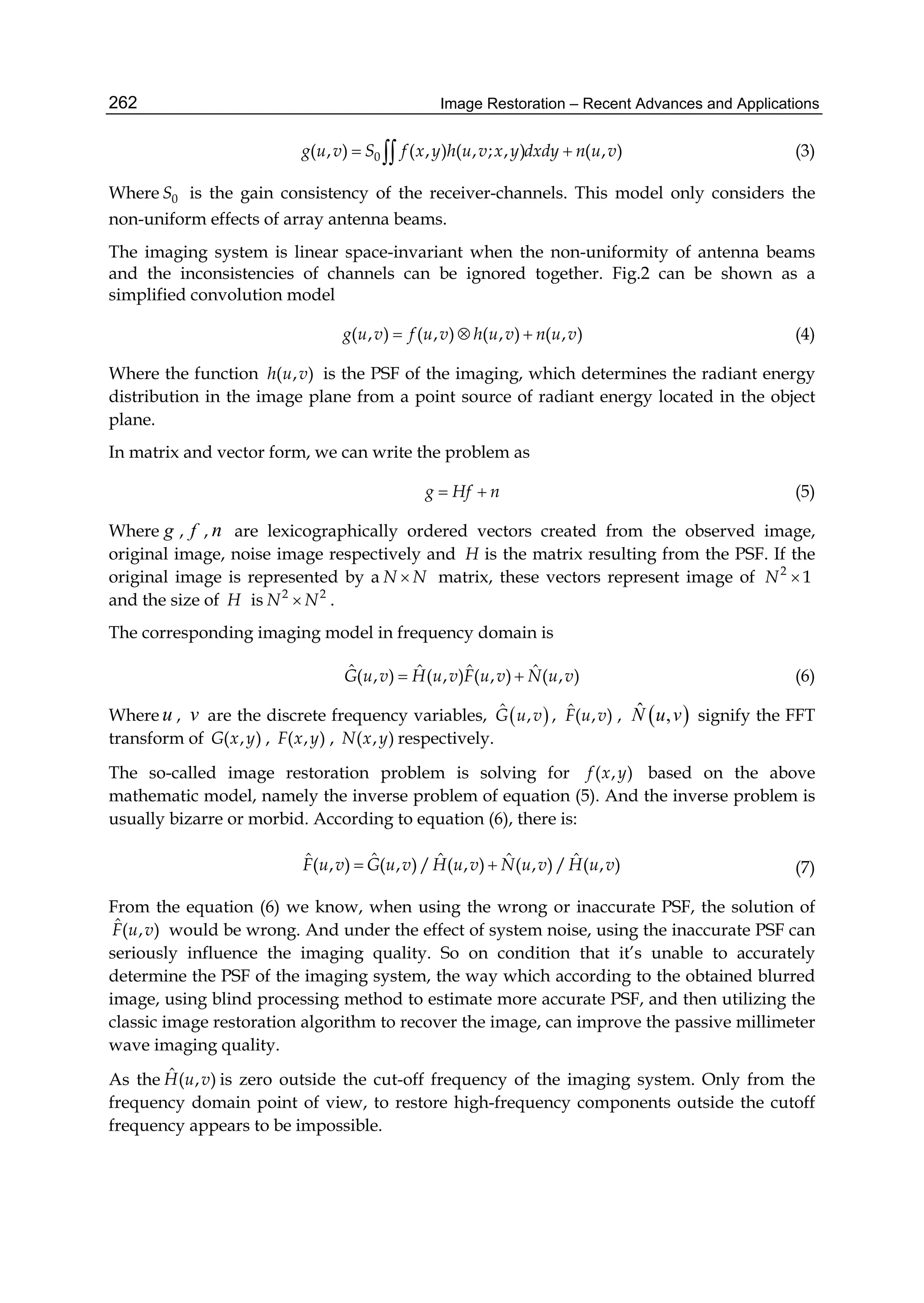
![Super–Resolution Restoration and Image Reconstruction for Passive Millimeter Wave Imaging 263
The analytical continuation theory is the theoretical basis for to achieve super-resolution.
Analytic continuation theory includes two aspects, 1) The Fourier transform of any airspace
bounded function is analytic functions. 2) For any analytic function, as long as we can
accurately know the part information in a limited range , we can uniquely determine the
entire function. Given the values of analytic function in a range, the overall reconstruction of
the function is called analytic continuation [21].
3. Variational bayesian estimate the PSF of the imaging system
In passive millimeter wave imaging signal processing, using accurate point spread function
(PSF) is important for getting high quality restored image. In the process of imaging, the PSF
is decided by antenna beam, atmospheric transmission, system noise etc. So the real PSF can
not be substituted by a simple model. We can't use a simple model to replace the real PSF.
And the PSF will change due to the specific imaging environment so that it is difficult to
acquire the exact PSF. The common methods to obtain the PSF include direct measurement
and model parameter estimation. In order to improve the quality of image restoration, a
variational Bayesian blind restoration algorithm for PMMW imaging is proposed in this
section, which combines the posterior probability model of the PMMW imaging to obtain
accurate point spread function by variational Bayesian estimation
The variational Bayesian estimation algorithm is based on Bayesian framework [22]. The idea
of this algorithm is according to the known priori information and assumptions establish a
posteriori distribution model of the imaging system first. And then under a certain criterion,
use the variational [23,24] method to obtain a optimal distribution which approximates with
the posteriori distribution, so that reducing the complexity of the model and make the problem
more analytic. Finally work out the estimation under the restriction of the cost function.
According to the Bayesian theorem, the posteriori distribution of passive millimeter wave
imaging system is decided by the prior distribution of original image, the prior distribution
of PSF, noise probability distribution and likelihood probability distribution. Because of the
prior distribution of original image is established on its gradient value of the statistical
distribution, according to the linear relationship of the above imaging model we can get
G( , ) ( , ) ( , ) ( , )x y H x y F x y N x y (8)
The is the gradient operator. Assuming that every point value of original image is
independent, , ( , )i jf F i j is the gradient value of each point. The prior distribution of
original image can be expressed by c-th order zero mean mixture gaussian distribution, the
mathematical expressed as
1, ,
( ) ( ) ( |0, )
C
i j c i j c
ci j i j
P F P f G f v
(9)
Where cv is the variance of the c-th Gaussian distribution, c is the weight of the c-th
Gaussian distribution.
Also, assuming that every point value of PSF is independent , ( , )m nh H m n is the point value
of the PSF. In passive millimeter wave imaging, the receive antenna’s power pattern is](https://image.slidesharecdn.com/imagerestorationrecentadvancesandapplications-160714160024/75/Image-restoration-recent_advances_and_applications-273-2048.jpg)
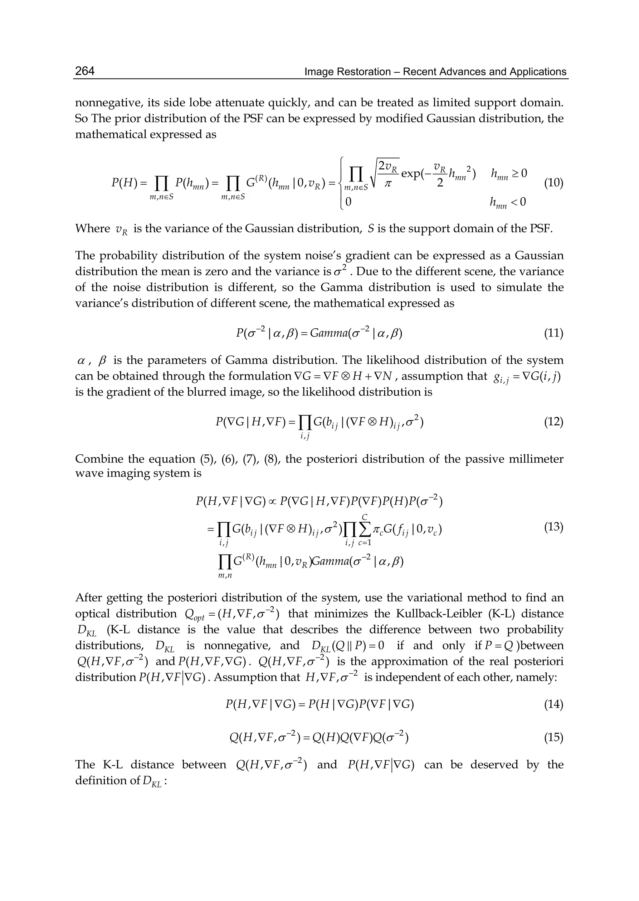
![Super–Resolution Restoration and Image Reconstruction for Passive Millimeter Wave Imaging 265
2
2
2 2
2
2 2
( , , )
( || ) log
( , | )
( , , )
( , , )log
( , | )
( , , ) ( )
( , , )log
( | , ) ( , )
KL
Q
Q H F
D Q P
P H F G
Q H F
Q H F dHd Fd
P H F G
Q H F P G
Q H F dHd Fd
P G H F P H F
(16)
Due to it is uncorrelated between ( )P G and 2
, ,H F
, so the new definition of K-L
distance is:
2
2
( , , )
( || ) log
( | , ) ( , )
( ) ( ) ( )
log log log
( ) ( ) ( | , )
KL
Q
Q
Q H F
D Q P
P G H F P H F
Q H Q F Q
P H P F P G H F
(17)
In order to minimize KLD , the minimum value can be deserved by partial derivate the
equation (13), so that we can get the ( )optQ H , the expression is:
2
( , | )
1
( ) ( )exp( log[ ( | , )] )opt Q F H
H
Q H P H P G H F
Z
(18)
Where HZ is a normalized variable. And then the optimum estimation of PSF can be
obtained by ( )optE Q H
.
The estimation ( )optQ H is not analytical, it has the form of ( ) exp( ( ))i i
i
P x a f x , so we can
use the iteration method to get the ( )optQ H . The solution procedure is as follows:
Obtain the parametric expression of ( )Q H from the form of the known ( )P H . Factor ( )Q H
into KLD , and get the update equations.Use the gradient descent method to get
the ( )optQ H .Get the expected value of ( )optQ H so that get the estimation of the PSF.
For PMMW imaging, the power pattern of the antenna is similar to gaussian function, so at
the beginning of the iteration we could use the gaussian function as its initial value, and
then through variational bayesian estimation to get more accurate PSF. That can reduce the
iteration times, and estimate the PSF faster.
According to the above analysis and derivation, the process of variational bayesian blind
restoration algorithm as shown in figure 3. First input blurred image and compute its
gradient value. Second set the initial value of variational bayesian iteration algorithm. Then
begin the variational bayesian estimation through the known priori information, when the
K-L distance less than the threshold, stop the iteration and output the estimated PSF. At last
use the Lucy-Richardson algorithm to restore the image, get the millimeter image of the
scene.](https://image.slidesharecdn.com/imagerestorationrecentadvancesandapplications-160714160024/75/Image-restoration-recent_advances_and_applications-275-2048.jpg)
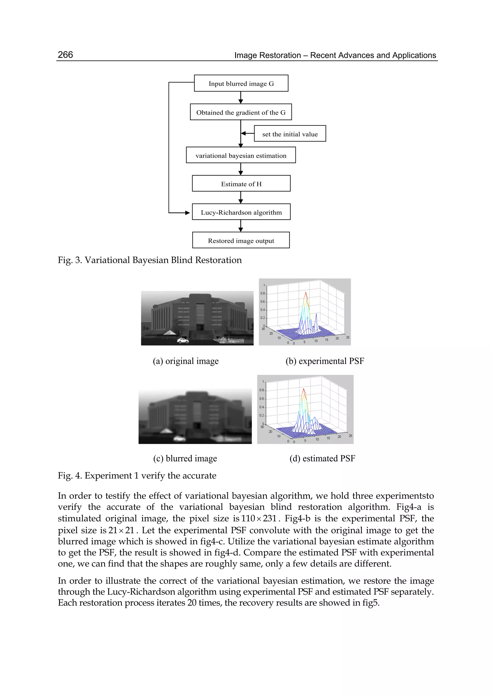
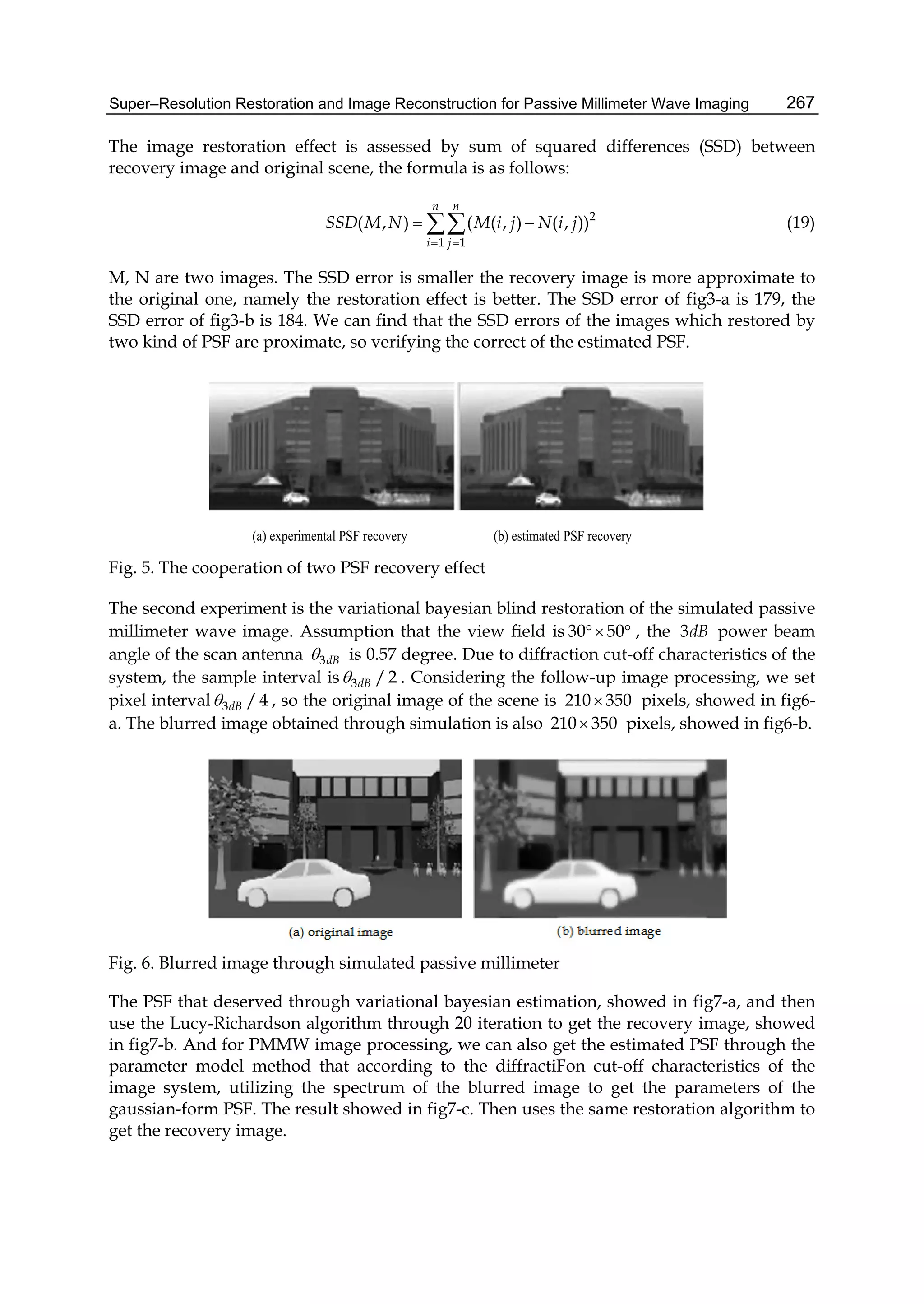
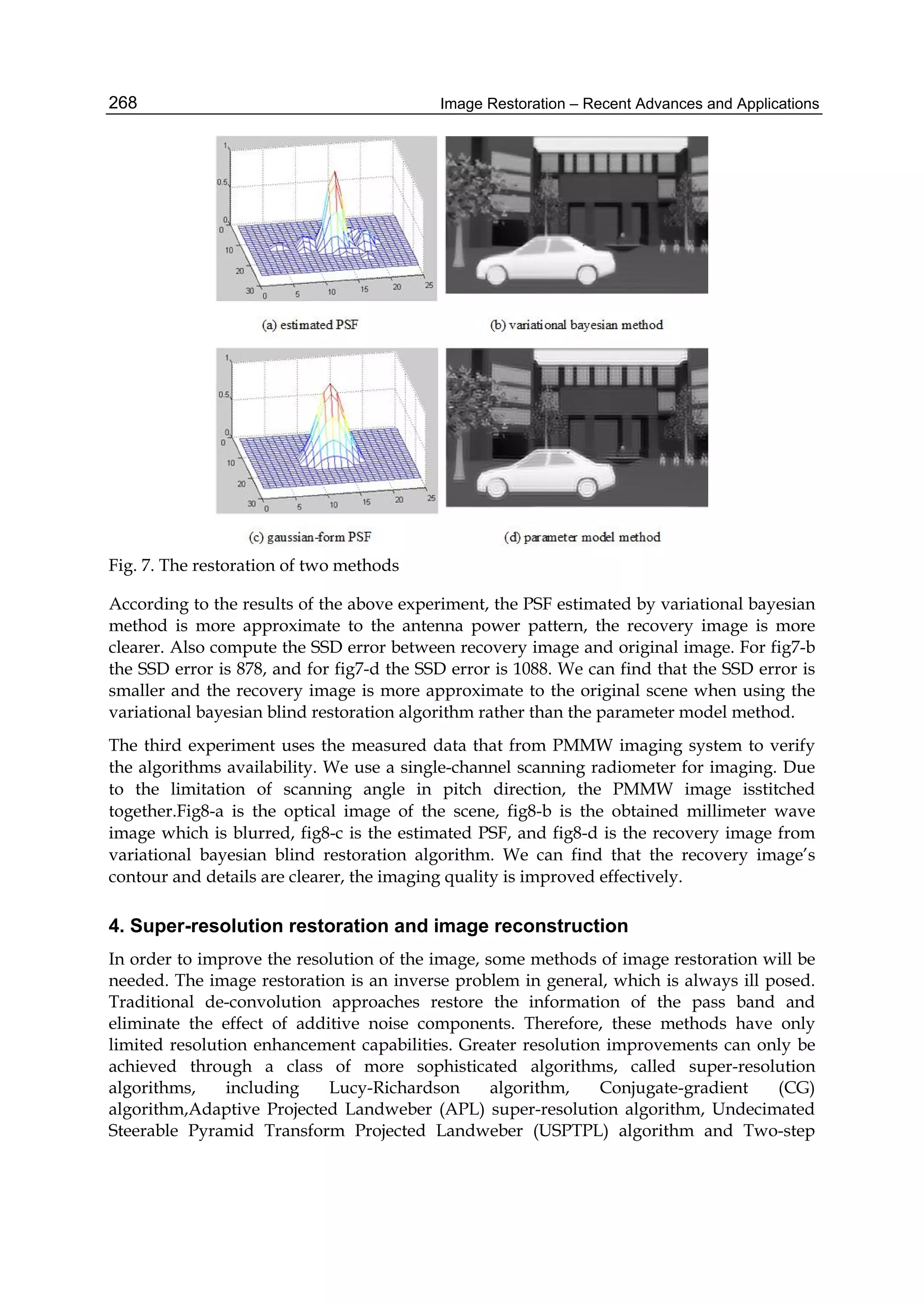
![Super–Resolution Restoration and Image Reconstruction for Passive Millimeter Wave Imaging 269
Projection Iteration Thresholding (tw-PIT) supper resolution using compressed sensing
architecture algorithm. In this section,wepresentthe image restoration algorithms.
(a) optical image (b) blurred image
(c) estimated PSF (d) recovery image
Fig. 8. Measured data restoration
Stochastic super-resolution image restoration, typically a Bayesian approach, provides a
flexible and convenient way to model a priori knowledge concerning the solution. Bayesian
estimation methods are used when the a posteriori probability density function (PDF) of the
original image can be established. Using maximum-a-posteriori estimation, we can obtain an
exact solution of the formula.
4.1 Conjugate-gradient algorithm
The Conjugate-gradient (CG) algorithm is an effective Krylov subspace method of solving
an unconstrained large-scale optimization problem, which is equivalent to solve the
quadratic minimization problem[25, 26].
2
1
min , 0
2
J Hf g f (20)
2
The target function can be denoted as
1 1
( )
2 2
T T T T
J f f H Hf g Hf H H (21)
And the gradient function is
( ( )) T T
grad J f H Hf H g (22)
The kf is the k-th iteration estimate of the original scene, it generates a descent direction kd ,
n~ is conjugate to all previous search directions: 1 2, ...... nd d d with respect to matrix T
H H ;
that is T T
n kd H Hd , k.=0,1,…n-1. In other words, conjugate gradient algorithm deals with
problem of 1D searching:](https://image.slidesharecdn.com/imagerestorationrecentadvancesandapplications-160714160024/75/Image-restoration-recent_advances_and_applications-279-2048.jpg)
![Image Restoration – Recent Advances and Applications270
1k k k kf f d (23)
where k denotes optimal size at searching directions, which is decided by
min ( ); ( )k k k k kJ f d d J f .
Because the standard conjugate gradient algorithm is a linear restoration method, it has only
limited capability of super-resolution, that is, spectral extrapolation. Furthermore, during
each iteration, we can not guarantee the nonnegative constraint of estimated images. An
interesting feature of the CG method is that it can be modified in order to take into account
the additional priori-information about the solution. The information can be expressed as a
number of closed convex sets.
An example of a constraint which is rather natural in many problems of image restoration is
the positivity of the solution. The constraint can also be projected as a closed convex set.
Thus we can impose the constraint that the image is nonnegative on the iteration. Because
the projection operation is non-linear operations, it introduces frequencies beyond the pass-
band. Thus, the modified CG algorithm has the capacity of spectrum extrapolation. It can be
shown as
1
1[ ]k
P C k k k kf P f f d
(24)
where cP denotes the projection operator on the constraint setC . Then the projection
operator is given by
0
0 0C
f if f
P f
if f
(25)
Other convex and closed sets include finite support constraint, band limited constraint, and
spatial limited constraint[27]. The super-resolution performance of the modified CG
algorithm can be verified from subsequent experiments.
Along with the increase of image size( n n ), the dimensions of matrix H is larger( 2 2
n n ),
it is bad for calculating and storage. However, H is Toeplitz matrix, a circulant convolution
matrix hB can be produced by H , it has features as follow[26]:
1
h hB W W
, * 1T
h hB W W
(26)
where
2
21
( , ) exp( ), , 0,1,... 1
j mn
W m n m n L
LL
, ( ( ))h diag DFT h (27)
The relationship between W, W-1and Discrete Fourier Transform (DFT) is as follows:
( ( ))Wp IDFT p n , 1
( ( ))W p DFT p n
(28)
In image processing, n is selected in the 2-power, such as 28-2128, etc. The amount of
calculation of image direct iteration restoring is very great at this time. However, H is
Toeplitz matrix(BTTB), so the matrix H (BTTB) can be continued to circulant matrix](https://image.slidesharecdn.com/imagerestorationrecentadvancesandapplications-160714160024/75/Image-restoration-recent_advances_and_applications-280-2048.jpg)
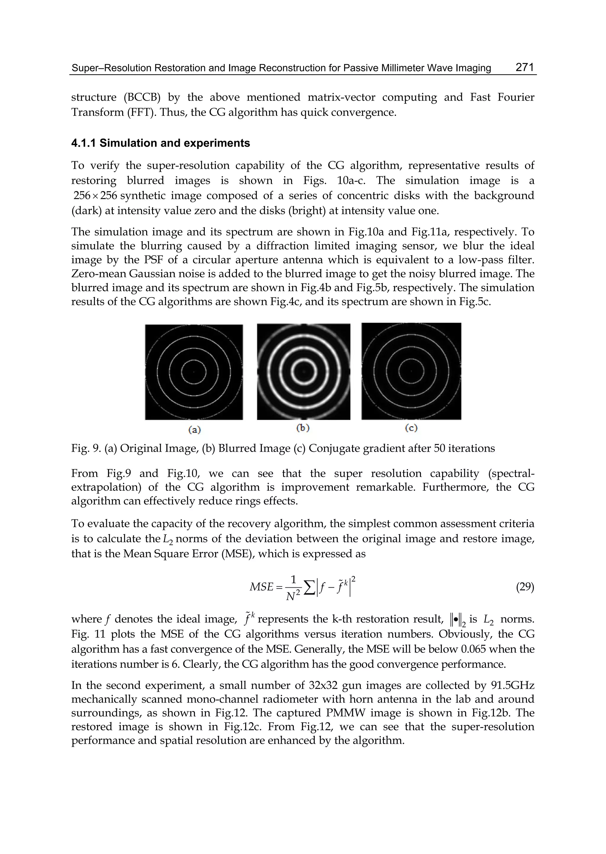
![Image Restoration – Recent Advances and Applications272
Fig. 10. Spectrum of Fig. 10 (a) Original Image, (b) Blurred Image (c) Result after CG
Fig. 11. MSE of the CG
(a) (b) (c)
Fig. 12. (a) Visible Image (b) Captured Image (c) Result of CG after 50 iterations
Experiment results demonstrate that the CG super-resolution algorithm has fast convergent
rate and the good spectral-extrapolation capacity. The CG algorithm improves the spatial
resolution and reduce the ringing effects which are caused by regularizing the image
restoration. Thus, the CG algorithm can be used in image restoration and PMMWI to
enhance the super-resolution performance and eliminate most of the effects of blurring.
4.2 Adaptive projected Landweber super-resolution algorithm
It is well-known that the problem of image restoration is the computation of f , given the
image data g and the PSF h . Some iterative methods have been introduced to solve
equation (5) [28]. Thebasic feature is that the number of iterations plays the role of a](https://image.slidesharecdn.com/imagerestorationrecentadvancesandapplications-160714160024/75/Image-restoration-recent_advances_and_applications-282-2048.jpg)
![Super–Resolution Restoration and Image Reconstruction for Passive Millimeter Wave Imaging 273
regularization parameter because semi-convergence holds true in the case of noisy images.
Iterative methods of image restoration have an advantage over one-step methods in that the
partial solution may be examined at each step of the iteration and any constraints on the
solution can be enforced at that time.
4.2.1 Landweber algorithm
The Landweber method (successive-approximation method) [29] is the simplest iterative
regularizing algorithm to solve linear ill-posed problems. Because standard Landweber
algorithm is a linear restoration method, it has only limited capability of super-resolution
(spectral extrapolation). Furthermore, during each iteration, we cannot guarantee the
nonnegative constraint of estimated image. Other disadvantages of the Standard Landweber
method are slow convergence and the difficulty of choosing proper update parameter.
Landweber algorithm is the simplest iterative method for approximating the least-square
solutions of equation (5). It is characterized by the equation
1
( )k k T k
f f H g Hf
(30)
Where T
H is the transpose of the blurring operator H ; superscript k denotes the
thk iteration; is a relaxation parameter controlling the convergence, in order to guarantee
the convergence of k
f , the value of are given by
2
1
2
0
(31)
Where 1 is the largest singular value of matrix H [30]. The initial guess 0
f is usually set to 0.
4.2.2 Projected Landweber super-resolution algorithm
Because standard Landweber algorithm is a linear restoration method, it has only limited
capability of super-resolution, that is, spectral extrapolation. Furthermore, during each
iteration, we cannot guarantee the nonnegative constraint of estimated image.
An interesting feature of the Landweber method is that it can be modified in order to take
into account additional priori information about the solution. Fundamental of reliable
estimation of high frequencies is the utilization of a priori known information during the
processing iteration. In fact, since image restoration is inherently an ill-posed problem, the
quality of restoration and the extent for achievable super-resolution depend on the accuracy
and the amount of a priori information. As shown there, many physical constraints on the
unknown object can be expressed by requiring that it belong to some given closed and
convex sets. While efforts at the modeling of constraint sets and the use of these in
projection-based set theoretic image recovery constitutes a popular direction for current
research, it seems that the idea of combining the strong point of Landweber schemes and
that of the projection-based methods has not been paid much attention to. The modified
Landweber method, also called the Projected Landweber Algorithm[31] is as follows
1 *
( )k k k
Cf P f H g Hf
(32)](https://image.slidesharecdn.com/imagerestorationrecentadvancesandapplications-160714160024/75/Image-restoration-recent_advances_and_applications-283-2048.jpg)
![Image Restoration – Recent Advances and Applications274
Where CP denotes the projection operator onto the constraint set C .
An example of a constraint which is rather natural in many problems of image restoration is
the positivity of the solution. We can impose the constraint that the image is nonnegative on
the iteration. Because this constraint is non-linear operation, it introduces frequencies
beyond the passband. The super-resolution performance of the Projected Landweber
algorithm can be verified from subsequent experiments. Then the projection operator is
given by
0
0 0C
f if f
P f
if f
(33)
Other convex and closed set C include finite support constraint, band limited constraint
and spatial limited constraint[27].
4.2.3 Adaptive projected Landweber Super-resolution alogithm
One disadvantage of the Landweber method is slow convergence and the difficulty to
choose proper update parameter. If is too large, the iterative process may diverge. If is
too small, the iterative process would be slow. Therefore, it is necessary to determine a
suitable for the iterative algorithm. Lie Liang and Yuanchang Xu proposed modification
of this method, Adaptive Landweber method [32], in which constant is calculated
adaptively in each iteration. The Adaptive Landweber algorithm has a better result and
faster convergence than standard Landweber algorithm. Instead of using a constant update
parameter, the Adaptive Landweber method computes the update parameter at each
iteration and chooses the maximum of the computed parameter and the preset
constantparameter to use in the next iteration.
Then we proposed a hybrid algorithm that attempt to combine the strong points of both
Projected Landweber scheme (simplicity of execution, Super-resolution, etc.) and the
Adaptive adjustments relax parameter (faster convergence rate, lower mean square error,
etc.). For a brief description, each cycle of this “Adaptive Projected Landweber algorithm”
consists of executing the three steps:
Step 1. Implement standard Landweber algorithm with initial relax parameter 0 and
0
0f
1
( )k k T k
kf f H g Hf
(34)
Step 2. Implement projection onto the convex set C
1 1k k
Cf P f
(35)
Step 3. Implement relax parameter 1k updating algorithm
1
2
1 0
2
max( , )
k
k k
f
f
(36)](https://image.slidesharecdn.com/imagerestorationrecentadvancesandapplications-160714160024/75/Image-restoration-recent_advances_and_applications-284-2048.jpg)
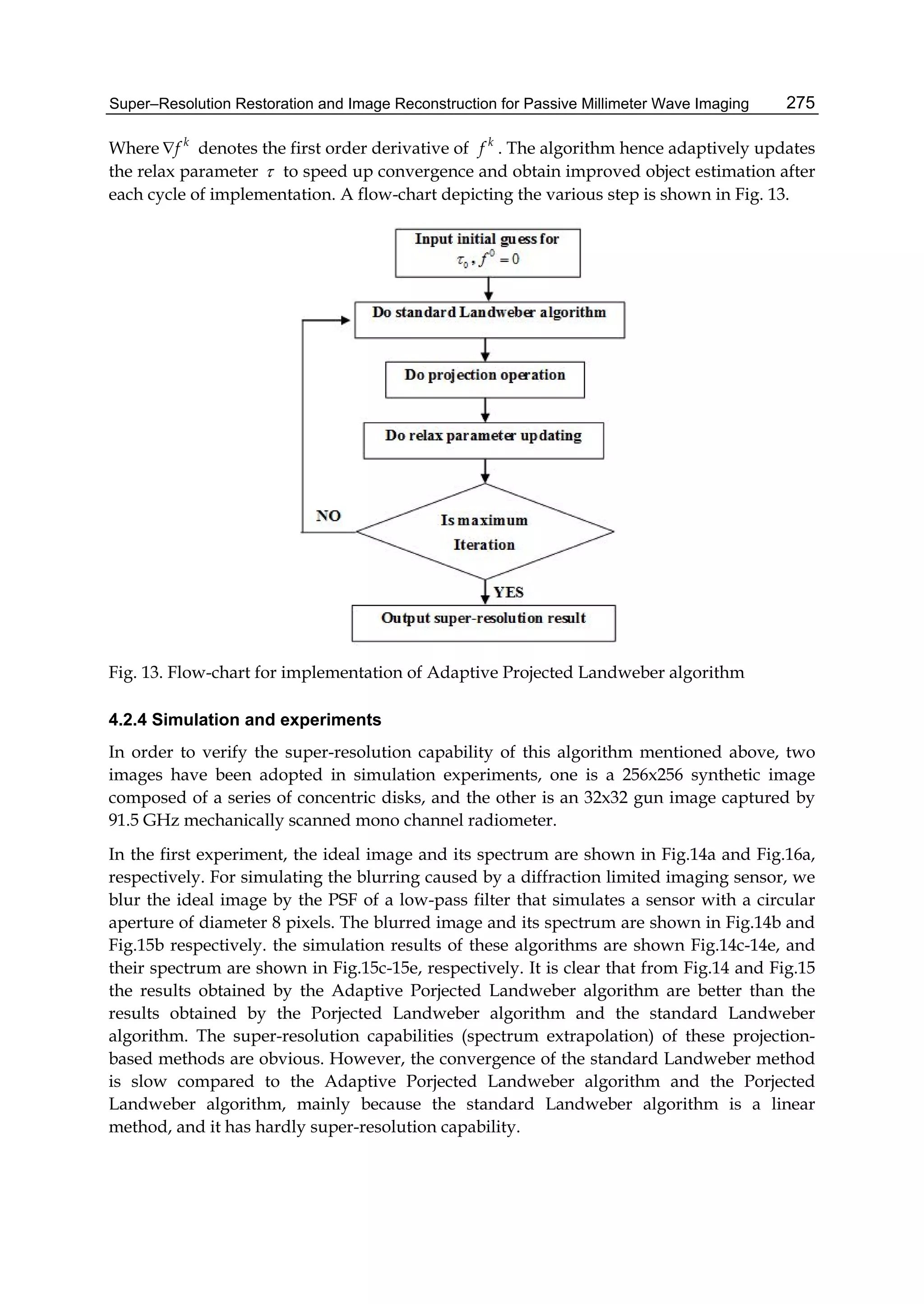
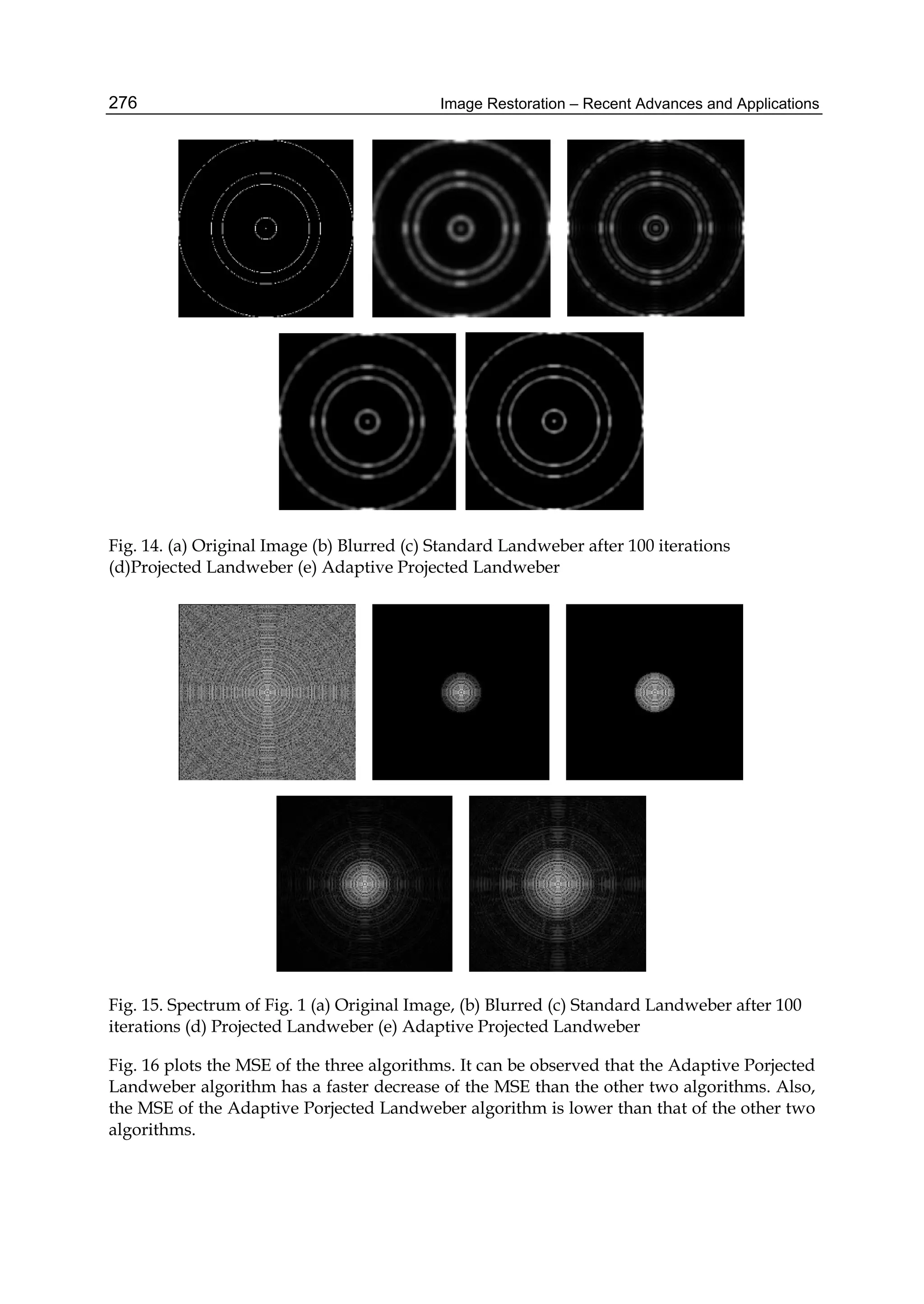
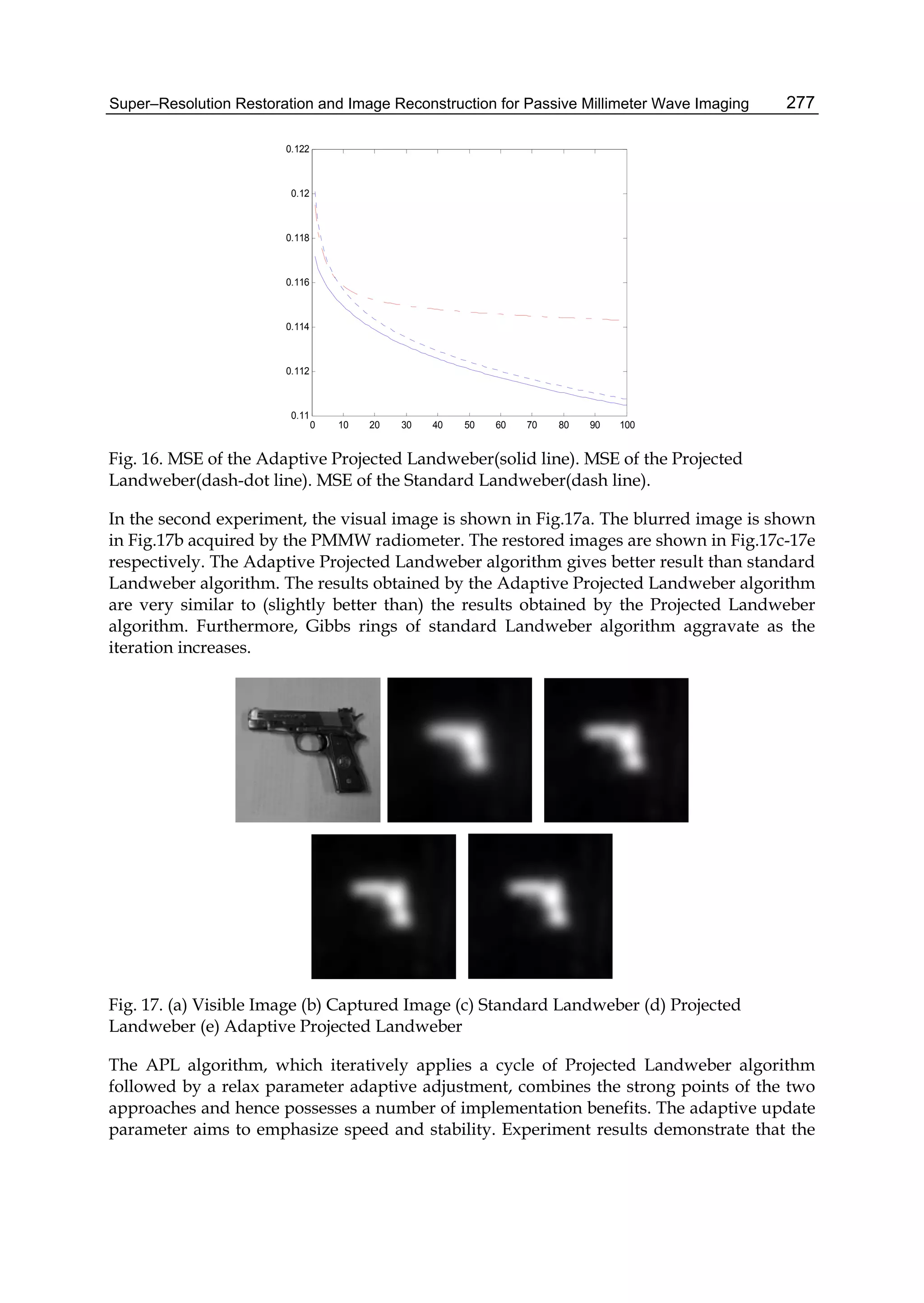
![Image Restoration – Recent Advances and Applications278
results of Adaptive Projected Landweber algorithm are better than those of standard
Landweber algorithm and Projected Landweber algorithm. The Adaptive Projected
Landweber Super-resolution algorithm has lower MSE and produces sharper images. These
constraints and adaptive character speed up the convergence of the Landweber estimation
process. The superior restoration of the object features observed in the image domain and
the significant extrapolation of spatial frequencies observed in the spectral domain lead to
the conclusion that the Adaptive Prejected Landweber super-resolution algorithm can be
used for restoration and super-resolution processing for PMMW imaging.
4.3 Undecimated steerable pyramid transform projected Landweber algorithm
Super resolution algorithms have two tasks: restoring the spectrum components within the
passband (by reversing the effects of convolution with the point spread function of imaging
system) and re-create the lost frequencies due to the imposition of sensor diffraction limits
by spectral extrapolation. Recently, a more sophisticated spectrum decomposition technique
is adopted. Using multi-scale technique, an image is decomposed into a hierarchical manner
where each level corresponds to a reduced-resolution approximation of the image. It is
equivalent to a filter bank that decomposes an image into different frequency components.
By such decomposition, one can restore the passband firstly and then extrapolate high
frequency components stage by stage. The most commonly used multi-scale methods are
based on the Pyramid transform (such as Laplacian Pyramid, steerable Pyramid), the
wavelets transform, the contourlets transform and so on [33-36]. The multi-scale transforms
mentioned above belong to linear transform, but they are not shift invariant due to the
down sampling. The lack of shift-invariance is a problem for many applications such as
image restoration and image denoising because it causes pseudo-Gibbs phenomena around
singularities [33]. Undecimated multi-scale methods can avoid such problem thus it has
been introduced in several studies [34-36].
4.3.1 Undecimated pyramid transform
The Undecimated Pyramid transform (UPT) uses filter bank ( 10H , 11H ) in the analysis part
and ( 10G , 11G ) in the synthesis part. The ideal frequency response of the building block of
the UPT is shown in Fig. 18(a). The perfect reconstruction condition is given as
10 10 11 11 1H G H G (37)
Filters of the UPT do not need to be orthogonal or bi-orthogonal and this lack of the need for
orthogonality or bi-orthogonality is beneficial for design freedom.
b
x
11H
10H
1y
2y
3y
21H
20H
x
11H
10G
11G
1y
2y
ˆx
10H
a
Fig. 18. Undecimated Pyramid transform. (a) The structure of the two-channel undecimated
filter bank (b) Two stage Pyramid decomposition.](https://image.slidesharecdn.com/imagerestorationrecentadvancesandapplications-160714160024/75/Image-restoration-recent_advances_and_applications-288-2048.jpg)
![Super–Resolution Restoration and Image Reconstruction for Passive Millimeter Wave Imaging 279
To perform the multi-scale decomposition, we construct non-subsampled pyramids by
iterated non-subsampled filter banks. For the next level, we upsample all filters by 2 in both
dimensions. Therefore, they also satisfy the perfect reconstruction condition. The cascading
of the analysis part is shown in Fig. 18(b).
Seen from frequency domain, the UPT decomposes an image into different frequency bands.
Suppose N is the order of the cascading decomposition, 0NH is a low frequency band and
1nH (1 )n N corresponds to high frequency component of the th
n stage. Let n be the
passband of 0nH , we have 1 2 3... . If the UTP is designed to acquire low
frequency component contained in , we can easily determine N by the inclusion relation
in frequency domain: 1N N .
In above mentionProjection Landweber algorithm, essentially the property of semi-
convergence indicates that the Landweber algorithm is a regularization method. Suppose a
perturbed linear equation is given as below
Ax b
(38)
Where A is an m n system matrix, which describes the system geometry, x is an 1n
vector of the image pixels and b
is an 1m vector of the measured data with perturbation
. Let kx
be the solution of equation (35) acquired by the Landweber after the th
k iteration,
kx be the solution of Ax b . If ( )b D A
, the Landweber algorithm has [37]
|| ||k kx x k
(39)
Where A
is the Moore-Penrose inverse of A . For a given , the data error || ||k kx x
is
amplified with the increase of iterative steps k . The algorithm stops at the semi-
convergence point when the data error reaches the magnitude of approaching error
|| ||kx x
, where x A b
.
Known from equation (36), the Landweber stops more quickly if it is used to restore an
image with a bigger . In the restoration of a badly contaminated image, the Landweber
may have not plenty iterative steps to restore or re-create the frequency components that we
need. Unfortunately, signal-to-noise ratio of PMMW image is quite low due to limited
integral time and bandwidth. Because of this, the PL algorithms can not provide a satisfied
resolution improvement in most practical applications. The practical performance of the PL
algorithm is shown in Fig. 23(c).
The denoising technique can avoid the fast termination of the Landweber algorithm.
Because PSF of a PMMW imaging system is approximately band-limited, a low passband
filter can perform the function. By such pre-procession, the high-frequency component of
is attenuated thus the Landweber algorithm avoid the adverse effect of the amplification of
high-frequency noise.
4.3.2 Undecimated Pyramid Projected Landweber (UPPL) super-resolution algorithm
The basic strategy of image super-resolution based on the UPT is to use a band-limit
frequency selection rule to construct a multilevel Pyramid-like restoration model from the](https://image.slidesharecdn.com/imagerestorationrecentadvancesandapplications-160714160024/75/Image-restoration-recent_advances_and_applications-289-2048.jpg)
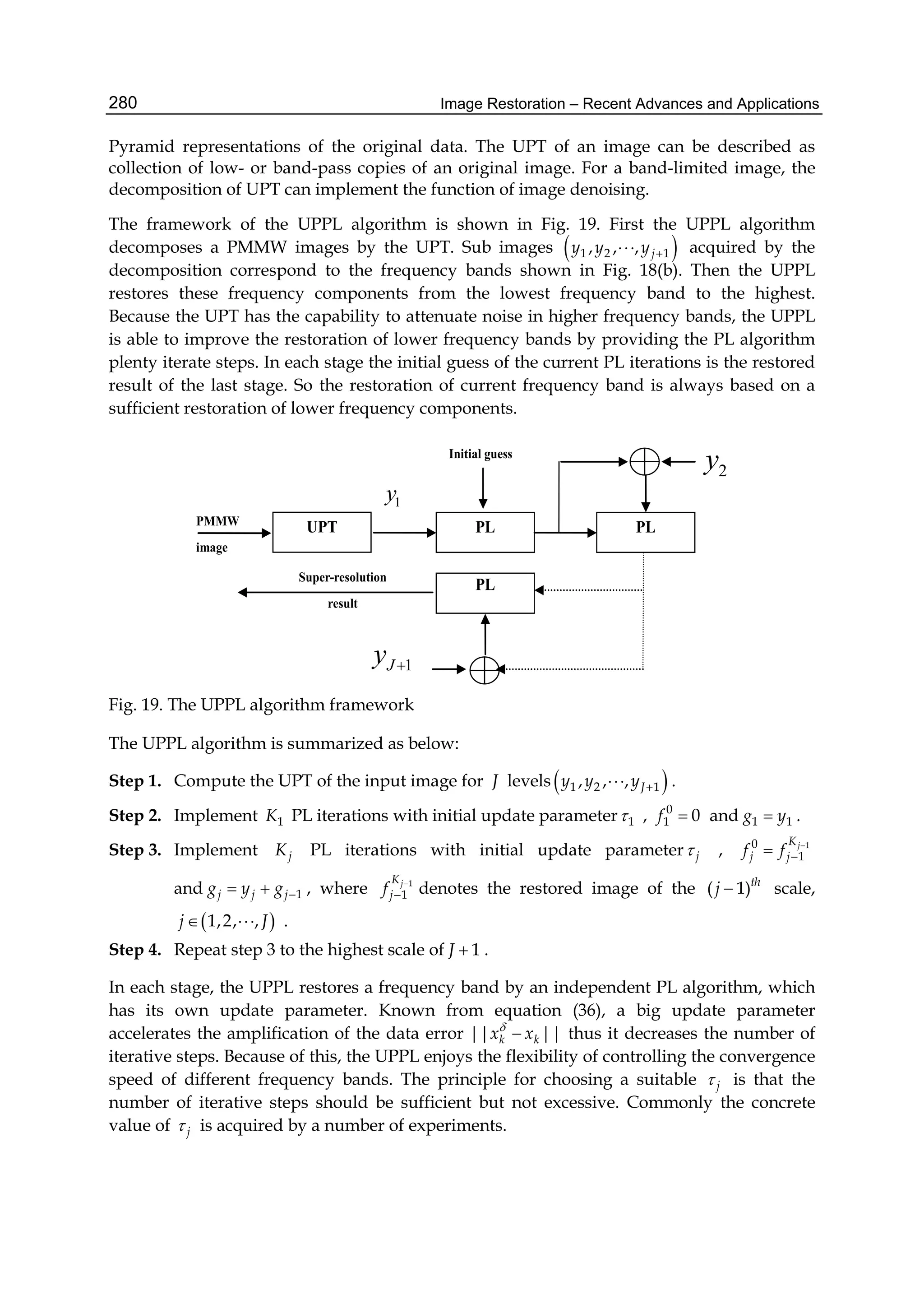
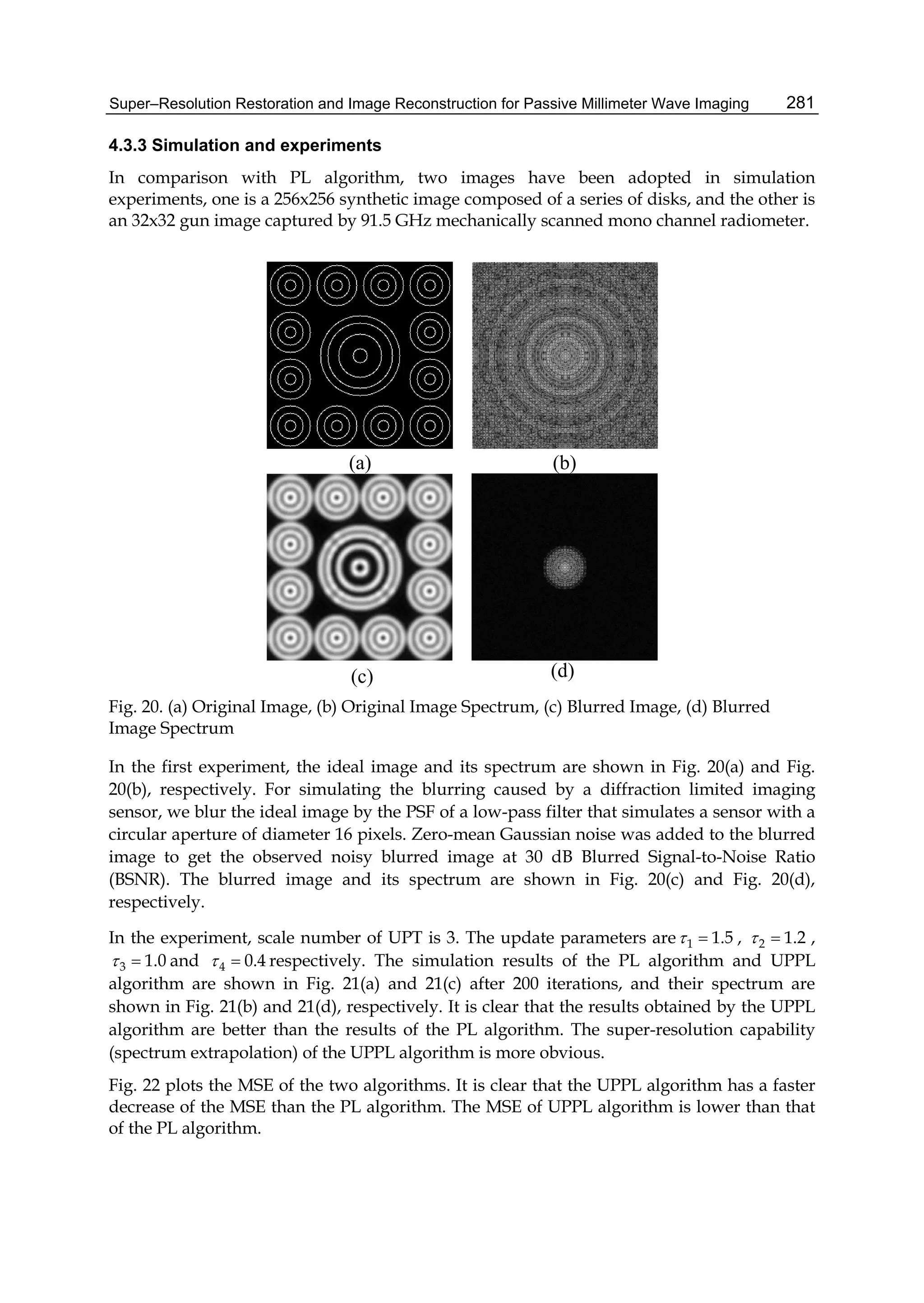
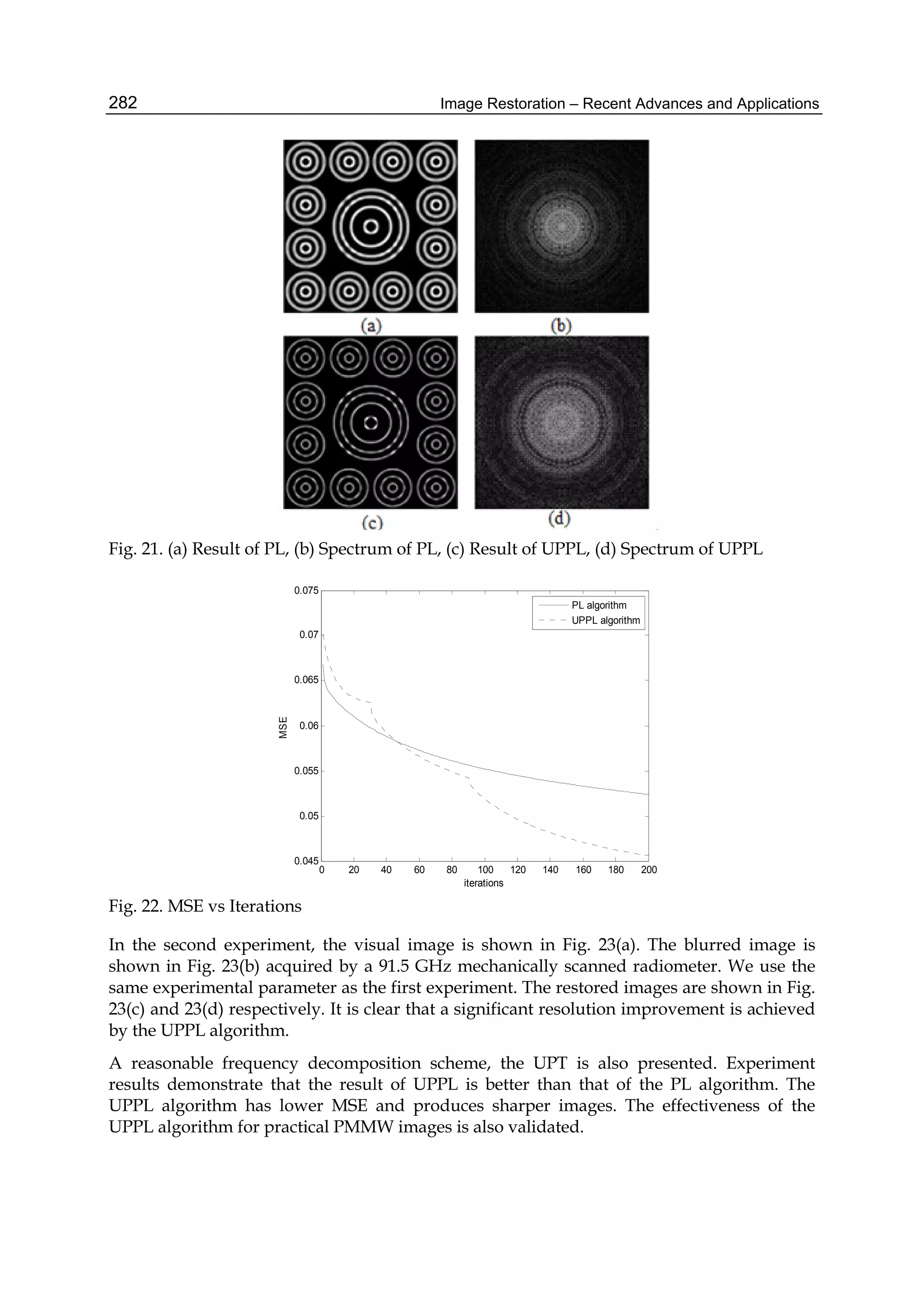
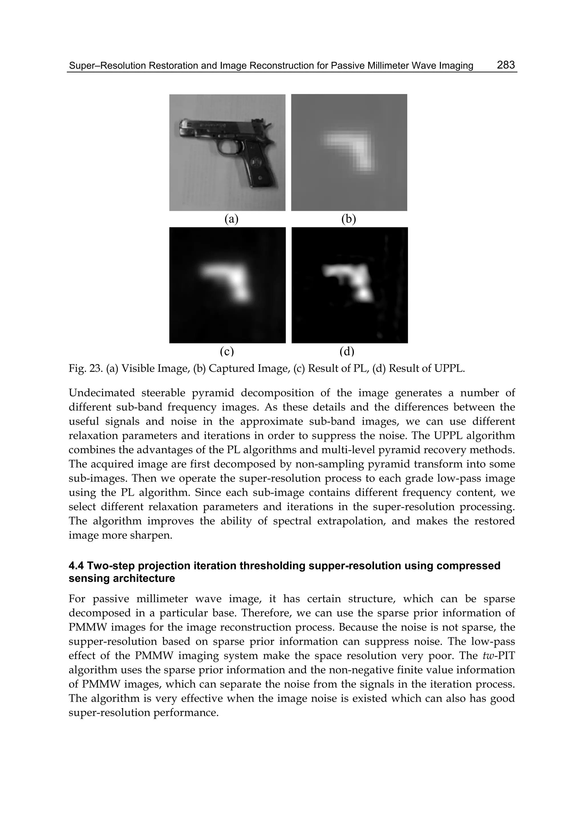
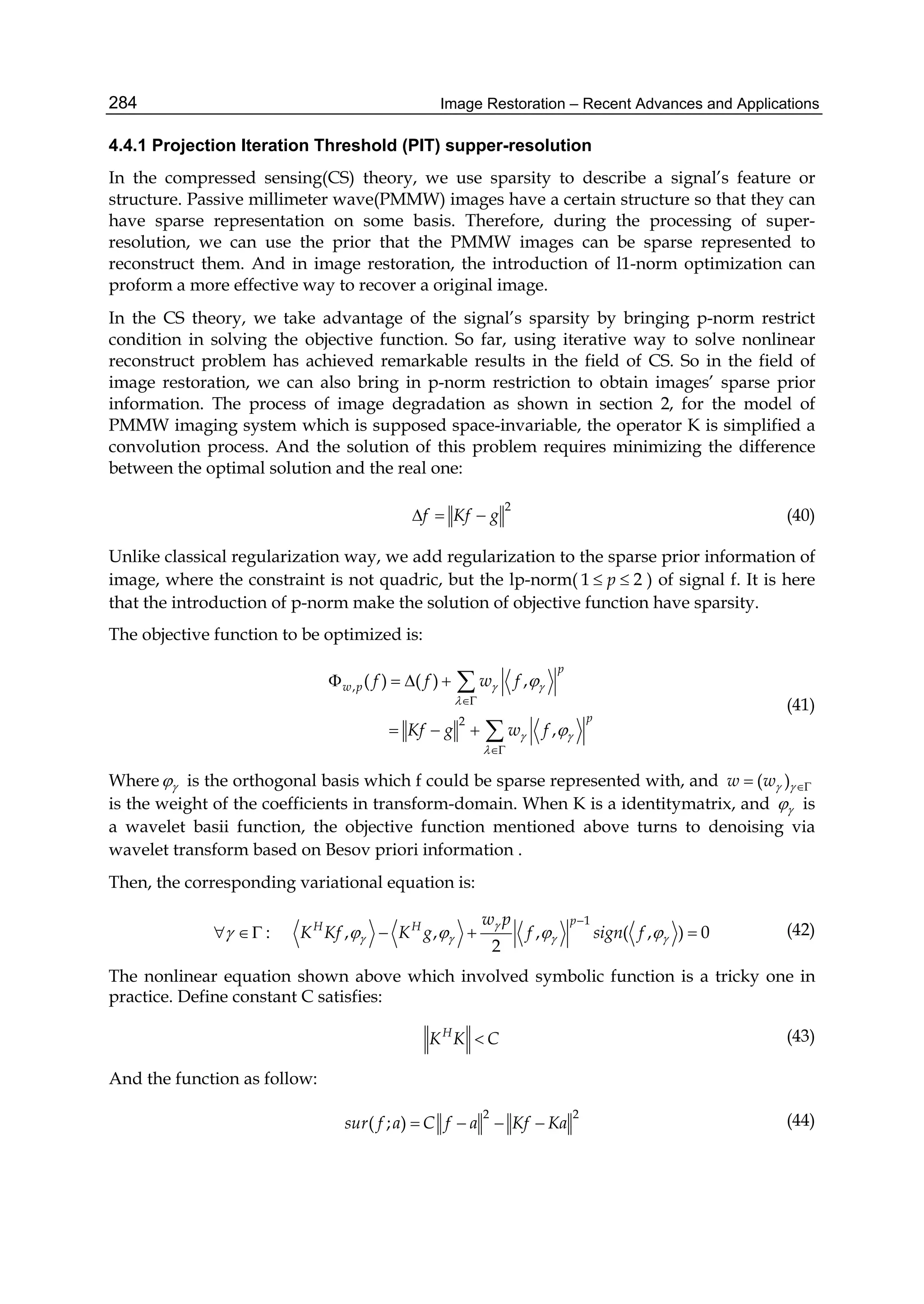
![Super–Resolution Restoration and Image Reconstruction for Passive Millimeter Wave Imaging 285
According the definition of C, H
CI K K is a strictly positive definite matrix. So function
( ; )sur f a is a strictly convex function for any value a. For image degradation, we can always
have 1K . So let C equal to value 1, and we can replace objective function by:
2 2
, ,
2
2 2 2
( ; )
[ 2 ( ) ]
sur
w p w p
pH H
f a Kf Ka f a
f f a K g K Ka w f
g a Ka
(45)
To acquire the solution of the equation above, the process of iteration is shown as follows.
For any initial point 0
f ,
1
,arg min( ( ; ) 1,2,...n sur n
w pf f f n
(46)
In equation (43), when w 0 , it means the objective function doesn’t include any sparse
priori information. Therefore, the algorithm is degraded to a process of landweber iteration
algorithm.
When p=1, the variational equation of the objective function is expressed as:
2 ( ) 2( [ ( ] )H
f w sign f a K g Ka (47)
For the process of symbolic function, when f >0, the solution is:
[ ( )] /2H
f a K g Ka w (48)
Under the condition of [ ( )] /2H
a K g Ka w , when f <0, the solution turns to:
[ ( )] /2H
f a K g Ka w (49)
otherwise, when the equation do not satisfy the two conditions mentioned above, which is
0f (50)
In conclusion, the iterating thresholding algorithm based on sparse prior is described as
follow
,1( [ ( )] )H
wf S a K g Ka (51)
Where ,1wS
is defined as follow:
,1
/2 /2
( ) 0 /2
/2 /2
i
w i
i
x if x w
S x if x w
x if x w
(52)](https://image.slidesharecdn.com/imagerestorationrecentadvancesandapplications-160714160024/75/Image-restoration-recent_advances_and_applications-295-2048.jpg)
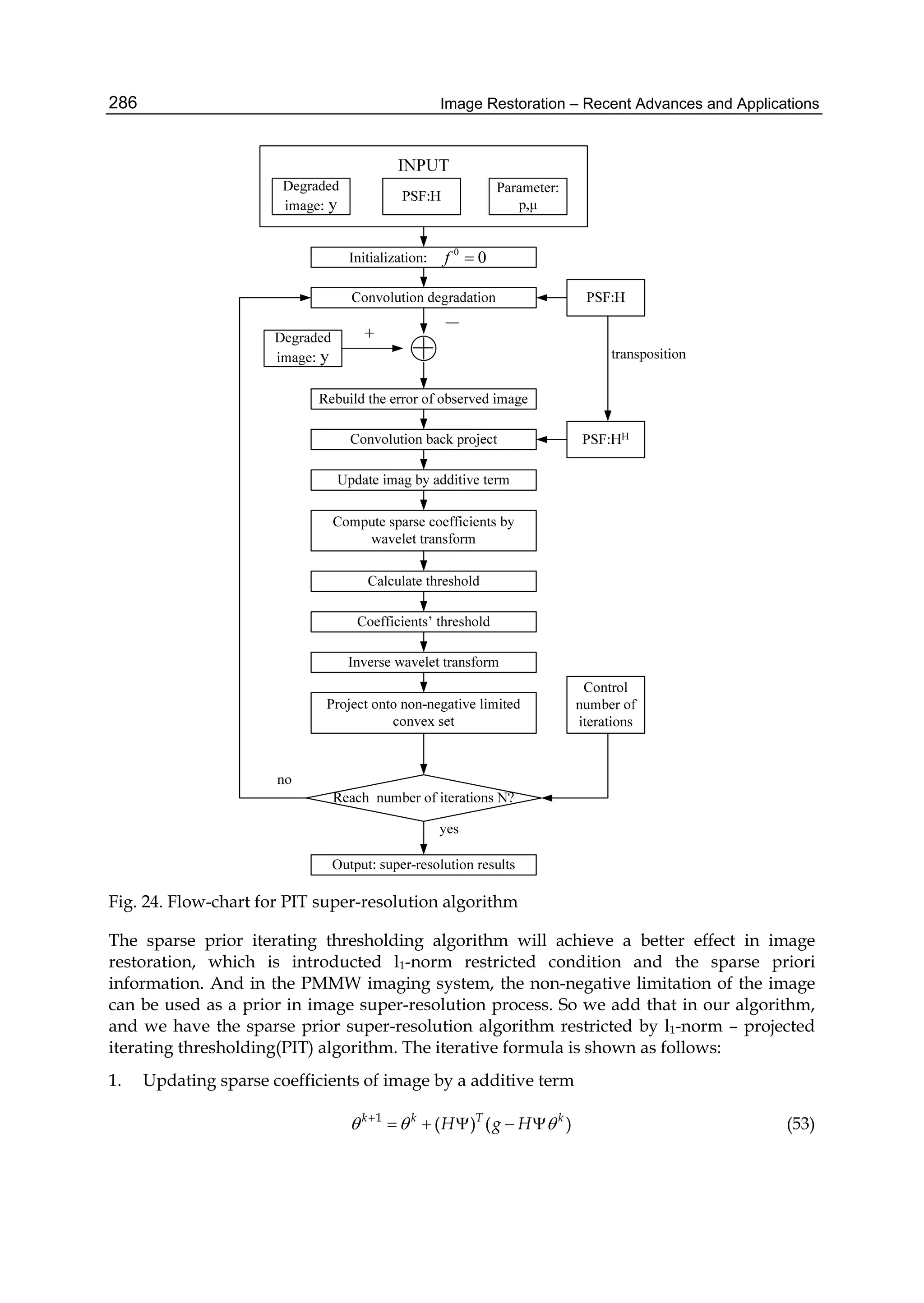
![Super–Resolution Restoration and Image Reconstruction for Passive Millimeter Wave Imaging 287
2. Computing soft threshold by the coefficients acquired above
1 1
1 1 1
1 1
/2 /2
( , ) 0 /2
/2 /2
k k
k k k
u
k k
S
(54)
3. Projecting onto a non-negative limited convex set
1 1
( )k k
Cf P
(55)
Where the definition of operator uS is soft threshold operation, and is the coefficient of
the image’s sparse representation on a certain orthogonal basis function.
Passive millimeter wave images can be sparsely represented. Assuming the orthogonal basis
is 1 2[ , ,..., ]N , the sparsity of image is expressed as follows:
f (56)
Where, f is the scene signal, is the sparse coefficient in orthogonal basis.
A flow chart depicting the various steps of Projected Iterating Thresh-holding (PIT) super-
resolution algorithm is shown as Fig. 24.
(a) (b)
(c) (d)
Fig. 25. (a) Original Image, (b) BlurredImage, (c) After Projected Landweber , (d) After twPIT](https://image.slidesharecdn.com/imagerestorationrecentadvancesandapplications-160714160024/75/Image-restoration-recent_advances_and_applications-297-2048.jpg)
![Image Restoration – Recent Advances and Applications288
After the above steps, one iteration is finished. Depending on the specific situation, the
algorithm can perform multiple iterations until reaching design requirement. The PIT
algorithm taking advantage of the sparse prior of the image, can have a better recovery
performance. Because of the isotropy, the noise has no sparsity in transform-domain. Since
we keep projecting to the l1-ball in every iteration, the algorithm can effectively eliminate
the impact of the noise’s amplification. We will verify it in the later simulation.
In one iteration, there are two convolutions of images, two wavelet transform operations,
two plus-minus operation and thresholding operation. The convolutions of images can
perform in frequency-domain, which could reduce calculations by using FFT, and wavelet
transform could achieve quickly by using Mallat algorithm.
4.4.2 tw-PIT supper-resolution
To improve the above algorithm, we can modify equation (52) by updating algorithm two-
step projection iteration [38-41]. Thus we can get two-step Projected Iterating Thresh-
holding, which is tw-PIT supper-resolution.
For a brief description, each cycle of this “tw-PIT supper-resolution algorithm” consists of
executing the four steps:
Step 1. The iterative principal process
1
( ) ( )k k T k
H g H
(57)
Where H is the PSF of system, g is the Captured PMMW image, is the sparse coefficient
in orthogonal basis .
Step 2. Soft threshold procedure:
1
/2 /2
0 /2
/2 /2
k k
i i
k k
i i
k k
i i
(58)
is the given parameters.
Step 3. Updating algorithm two-step projection iteration
1 1 1
(1 ) ( )k k k k
f f f
(59)
The designation “two-step” stems from the fact that depends on both k
f and 1k
f
, rather
than only on k
f .
Step 4. Projection process
1 1
( )k k
Cf P f
(60)
Where
2
1
2 2
,
1 1 N
, 1
1
, 1N
N
N
, 1 can be 0.1,0.01,0.001,0.0001, et al.](https://image.slidesharecdn.com/imagerestorationrecentadvancesandapplications-160714160024/75/Image-restoration-recent_advances_and_applications-298-2048.jpg)
![Super–Resolution Restoration and Image Reconstruction for Passive Millimeter Wave Imaging 289
Tw-PIT supper-resolution algorithm can finish one iteration though the above four steps.
The algorithm converges very fast. The convergence is much faster with 1 is much smaller.
But it does not guarantee optimal performance of the reconstruction algorithm.
4.4.3 Simulation and experiments
In order to verify the super-resolution capability of thetw-PITalgorithm mentioned above,
two images have been adopted in simulation and experiments, one is a lena image, and the
other is an 210×96 University of ElectronicScience and Technology of China (UESTC)
library’s image captured by 94 GHz mechanically scanned mono channel radiometer.
In the first experiment, the optical lena image and the blurred image are shown in Fig.25a
and Fig.25b respectively. The blurred image is from the lena image via a 5×5 Gaussian
templates convolution. Zero-mean Gaussian white noise is added to the blurred image. The
noise variance is 10. The Blurred Signal-to-Noise Ratio (BSNR) is 30 dB of the noisy blurred
image. The experimental parameters 1 is 0.1. The results obtained by the Projected
Landweber and twPIT are shown in Fig.25c and Fig.25d. This metric is given by[42]
2
,
10 2
1
( , ) ( , )
10 log ( )
i j
y i j y i j
MN
BSNR
(61)
Where, , , ,y i j g i j n i j is the noise free blurred image, ( , )y m n E y , 2
is the
additive noise variance.
It is clear from Fig.25 that the results obtained by the twPIT algorithm are better than the
results obtained by the PL algorithm.
When the ideal image is available for comparison, various distance metrics can be readily
postulated to compare the images and their spectra. Straightforward measure is the Mean
Square Error (MSE), which given by
2
2
1 k
MSE f f
N
(62)
Where f denotes the ideal image, k
f represents the thk restoration result, 2
is 2L norms.
Fig. 26 plots the MSE of the three algorithms.
It can be observed that the twPIT algorithm has a faster decrease of the MSE than the PL
algorithm and PIT algorithm from Fig.27. Also, the MSE of the twPIT algorithm is lower
than that of the other two algorithms. Clearly, the twPIT algorithm has the best convergence
performance and lowest MSE. This is because the twPIT algorithm suppress the noise in an
iterative process. The experiments show that the twPIT algorithm convergence faster, which
is suitable for the required real-time applications, such as airport security and Concealed
Weapons Detection.
In the second experiment, the visual image is shown in Fig.28a. The PMMW image is shown
in Fig.28b, which is captured by a 3mm Passive millimeter wave focal plane linear array
scanning imaging system. The restored images are shown in Fig.28c-28e, respectively. Fig.27](https://image.slidesharecdn.com/imagerestorationrecentadvancesandapplications-160714160024/75/Image-restoration-recent_advances_and_applications-299-2048.jpg)
![Image Restoration – Recent Advances and Applications290
is the PSF which is estimated by variational bayesian. In captured image, the image are
assembled together by three times mechanically scanned mono-channel radiometer, as a
single mechanical scan pitch direction field limit.
Fig. 26. Mean square error of the reconstructed image
Fig. 27. Variational bayesian estimated PSF
The MSE is a global evaluation criterion for super-resolution algorithm. We can use the local
image variance method to estimate the image noise level. This approach is based on the
assumption, which the image is a large number of small pieces of uniform composition, and
image noise to additive noise based. The captured passive millimeter wave images meet this
requirement, which there are many flat background and noise is mainly additive noise,
basically meet the above assumptions. Local variance calculated as follows [43]:
1. The image is divided into many small block, such as 4×4, 5×5. Then, we calculated the
local mean and local variance of each block. The local variance is defined as:
2 21
( , ) [ ( , ) ( , )]
(2 1)(2 1)
QP
y y
k P l Q
i j y i k j l i j
P Q
(63)](https://image.slidesharecdn.com/imagerestorationrecentadvancesandapplications-160714160024/75/Image-restoration-recent_advances_and_applications-300-2048.jpg)
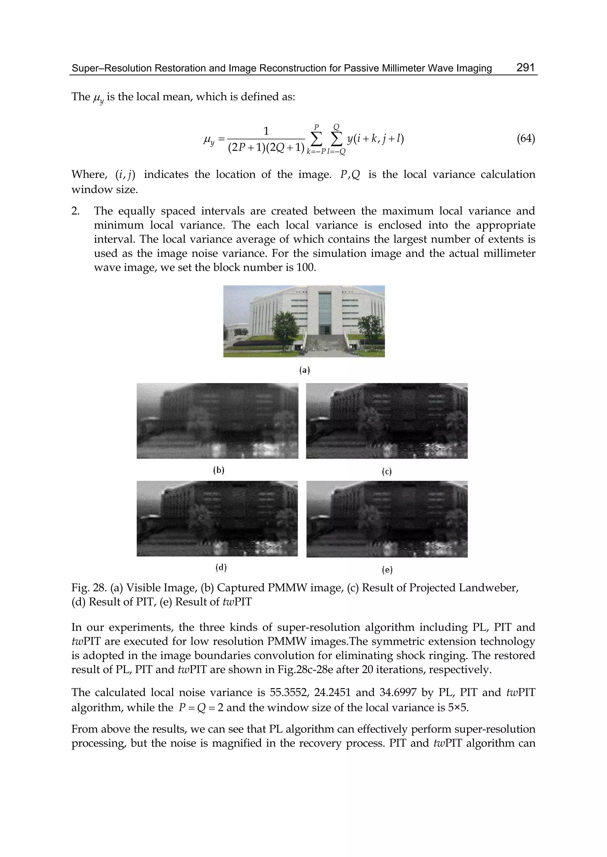
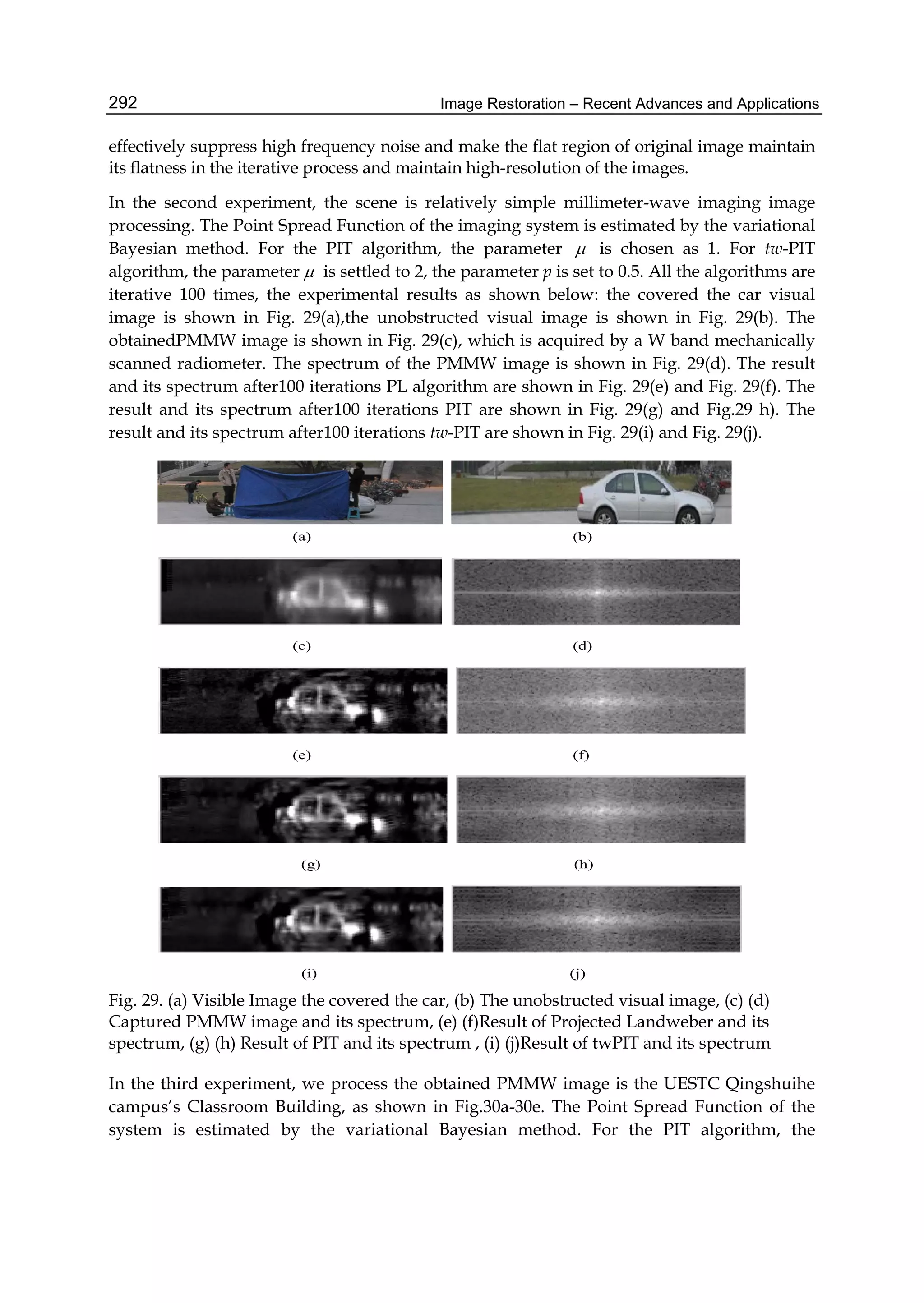
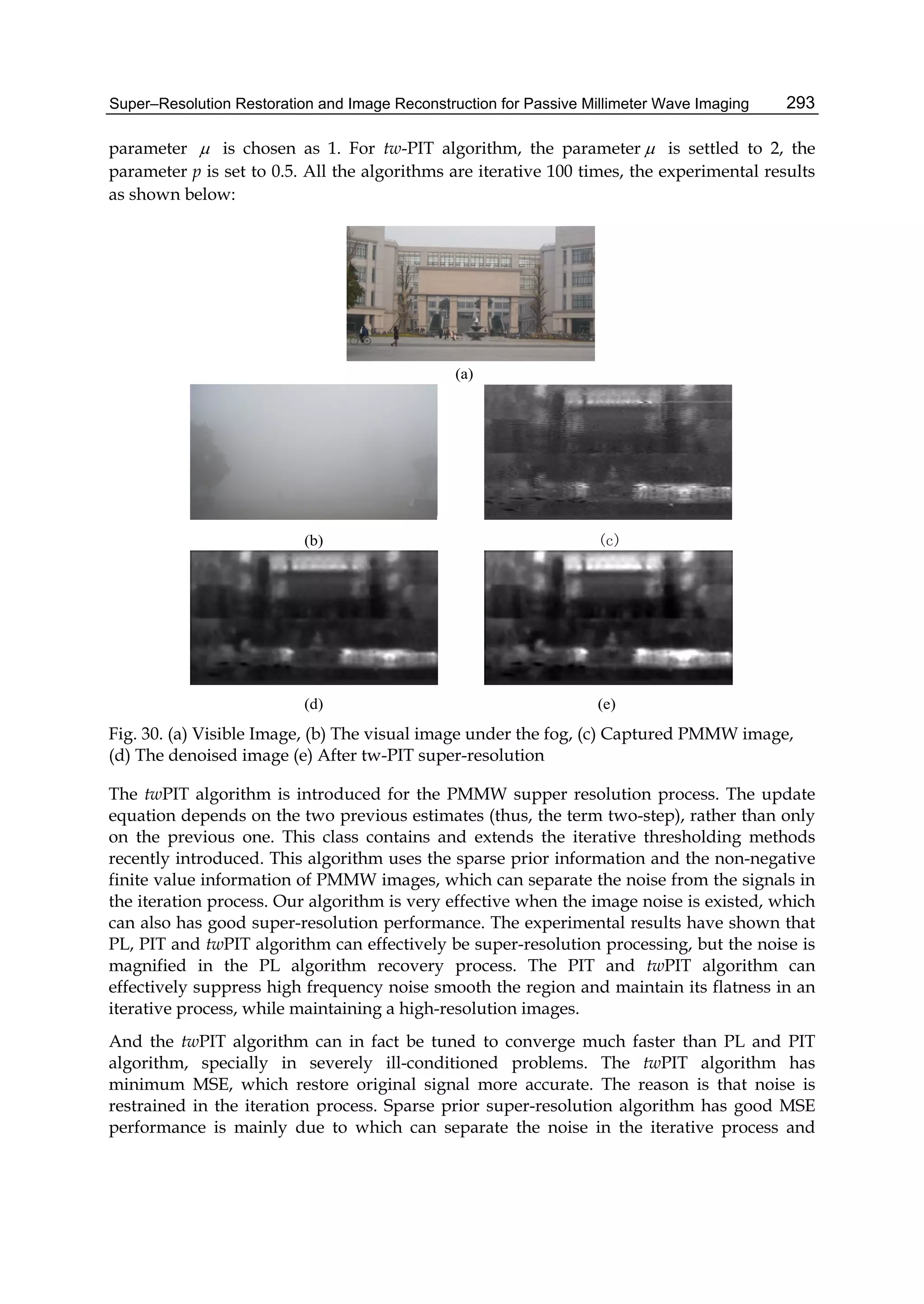
![Super–Resolution Restoration and Image Reconstruction for Passive Millimeter Wave Imaging 295
Zelong Xiao, Jianzhong Xu, Shusheng Peng, et al. “Super resolution image restoration of a
PMMW sensor based on POCS algorithm. Systems and Control in Aerospace and
Astronautics, ” 2006. ISSCAA 2006, 2006, 680-683
L. C. Li, Research on Passive Millimeter Wave Imaging Theory and Super-resolution Signal
Processing Technology, Ph.D. dissertation, Dept. of Electronic Engineering,
University of Electronic Science and Technology of China, 2009.
L. C. Li, J. Y. Yang, J. T. Xiong, et al., “W Band Dicke-Radiometer For Imaging,” Int J
Infrared Milli Waves, 29:879–888(2008).
L. C. Li, J. Y. Yang, et al., “Method of passive mmW image detection and identification for
close target,” Int. J. Infrared Milli. Waves, (2011) 32: 102-115.
L. C. Li, J. Y. Yang, et al., Research on 3mm radiometric imaging, Journal of infrared and
millimeter waves, Vol.28(1):11-15, 2009.
L. C. Li, J. Y. Yang, et al., An Focal Plane Array Space Variant Model For PMMW Imaging,
IET International Radar Conference 2009.
Goodman, J.W. Introduction to Fourier Optics 2nd.(McGraw-Hill Book Co, New York, 1996)
Su Bing-hua, Jin Wei-qi, Niu Li-hong, NIU Li-hong, LIU Guang-rong. Super-resolution
image restoration and progress. Optical Technique, 2001, 27(1):6-9.
Steven M. Kay.Fundamentals of Statistical Signal Processing, Volume I: Estimation Theory
and Volume :Detection Theory [M]. Beijing: Publishing House of Electronics
Industry, 2003.
Sina Farsiu, M. Dirk Robinson,and et al. “Fast and Robust Multiframe Super Resolution”,
IEEE Trans. On Image Process, 2004, 13(10), pp. 1327–1344.
A. Chambolle. "Total variation minimization and a class of binary MRF models", Proc. Int.
Workshop on Energy Minimization Methods in Computer Vision and Pattern
Recognition, 2005,Vol 3757,pp.136-152.
Kyung Sub Joo, Tamal Bose, and Guo Fang Xu. Image restoration using a conjugate gradient
based adaptive filtering algorithm. Circuits system signal processing, 1997,16 (2)
:197-206.
Zou Mouyan. Deconvolution and Signal Recovery [M. Beijing: National Defence Industry
Press, 2001
Stark H. “Image recovery: theory and application,” New York:Academic Press, 1987.
J. Biemond, R. L. Lagendijk, R.M.Mersereau, “Iterative methods for image deblurring,”
Proc.of IEEE, Vol.78, pp.856-883, 1990.
L. Landweber. “An iteration formula for Fredholm integral equations of the first kind,”
American Journal of Mathematics, vol 73, pp 615–624, 1951.
R. W. Schafer, R. M. Mersereau, and M. A. Richards, “Constrained iterative restoration
algorithms,” Proc. IEEE, vol. 69, pp. 432-450, 1981.
Piana M, Bertero M. “Projected Landweber method and preconditioning,” Inverse Problems,
Volume 13, Issue 2, pp. 441-463,1997.
Lei Liang and Yuanchang Xu, “ Adaptive Landweber method to deblur images,” IEEE
Signal Processing Letters, Vol. 10, No. 5, 2003.
Marta Peracaula, Joan Martí, Jordi Freixenet, etc. Multi-Scale Image Analysis Applied to
Radioastronomical Interferometric Data, Pattern Recognition and Image Analysis,
Vol. 5524, 2009, pp. 192-199.](https://image.slidesharecdn.com/imagerestorationrecentadvancesandapplications-160714160024/75/Image-restoration-recent_advances_and_applications-305-2048.jpg)
![Image Restoration – Recent Advances and Applications296
Eslami R, Radha H. Translation-invariant contourlet transform and its application to image
denoising. IEEE Transactions on image processing, Vol. 15, No. 11, 2006, pp. 3362 –
3374.
A. L. Cunha, J. Zhou, and M. N. Do, The non-subsampled contourlet transform: Theory,
design, and applications, IEEE Transactions on Image Processing, Vol. 15, No. 10,
2006, pp. 3089-3101.
J.-L. Starck, J. Fadili, and F. Murtagh, The undecimated wavelet decomposition and its
reconstruction, IEEE Trans. Image Processing, Vol. 16, No. 2, 2007, pp. 297-308.
Wang Yanfei, Computational methods for inverse problems and their applications. Higher
education press of China, 2005.
I Daubechies, M Defrise, C De Mol.An iterative thresholding algorithm for linear inverse
problems with a sparsity constraint[J]. Comm.Pure Appl.Math., 2004, 57(11):1413-
1457.
Emmanuel Candes and Terence Tao. “Near optimal signal recovery from random
projections Universal encoding strategies”, IEEE Trans. on Information Theory,
2006, 52(12), pp. 1-39.
J. Bioucas-Dias and M. Figueiredo, “A new TwIST: Two-step iterative
shrinkage/thresholding algorithms for image restoration”, IEEE Trans. Image
Process, 2007, 16(12), pp. 2992–3004.
A. Beck and M. Teboulle. “A fast iterative shrinkage-thresholding algorithm for linear
inverse problems”. SIAM Journal on Imaging Sciences, Mar 2009, 2(1):183-202.
Bahnam M A , Katsaggelos A K. Digital image restoration[J]. IEEE Signal Process. 1997,
14(2): 24–41.
Gao B C. An OperationalMethod for Estimating Signal to Noise Ratios from Data Acquired
with Imaging Spectrometers. Remote Sensing of Environment, 1993, 43 (1):23—33.](https://image.slidesharecdn.com/imagerestorationrecentadvancesandapplications-160714160024/75/Image-restoration-recent_advances_and_applications-306-2048.jpg)
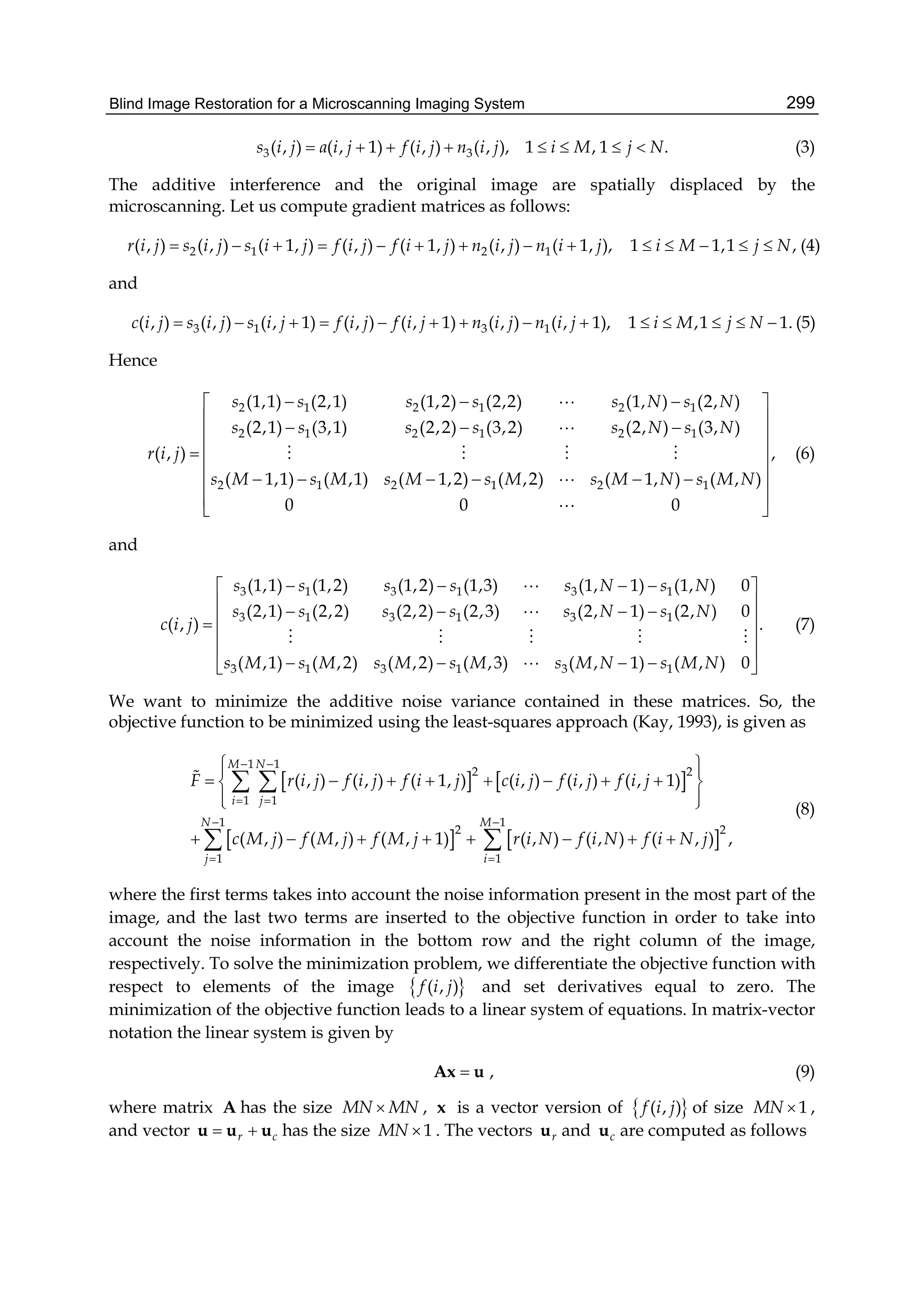
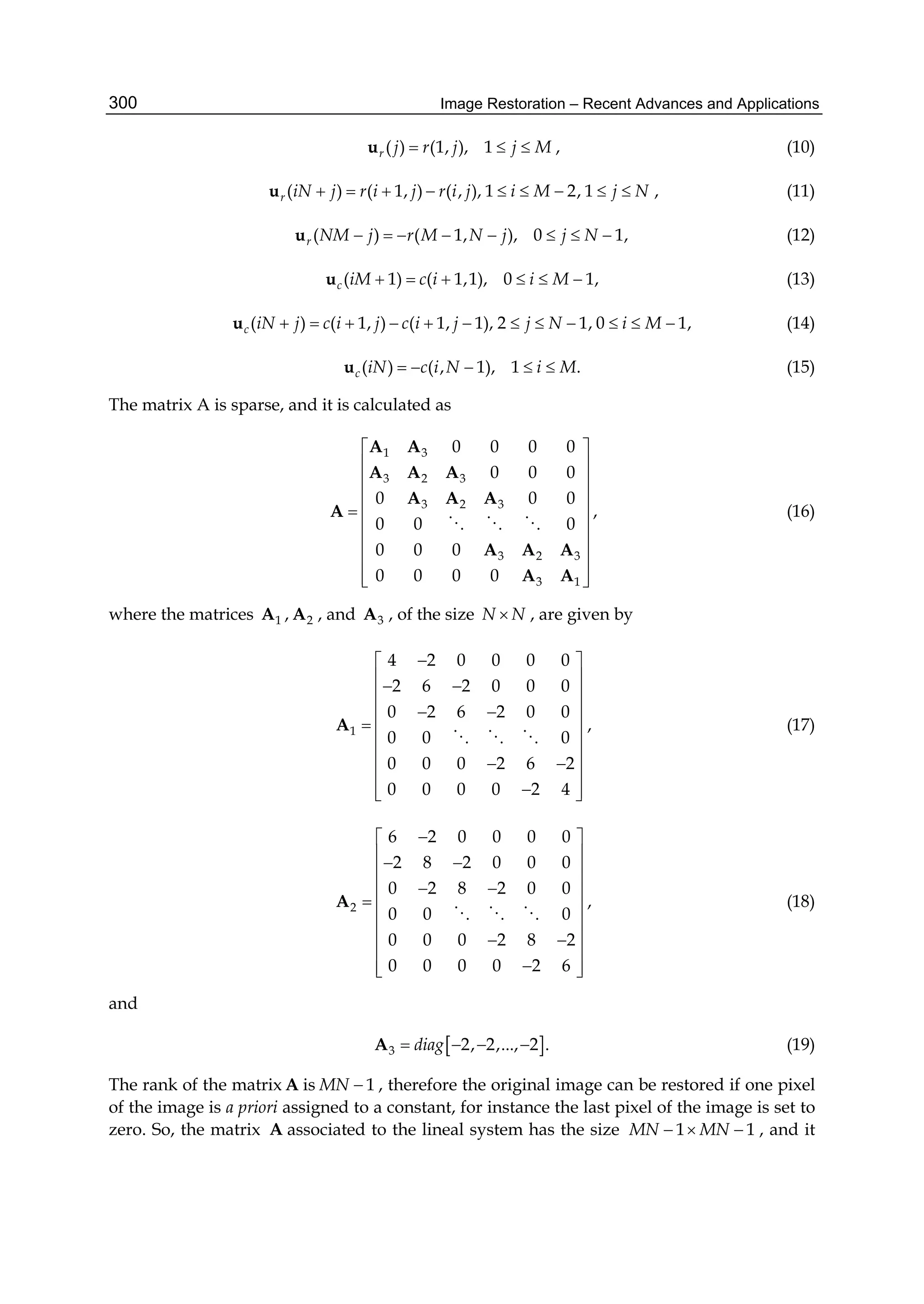
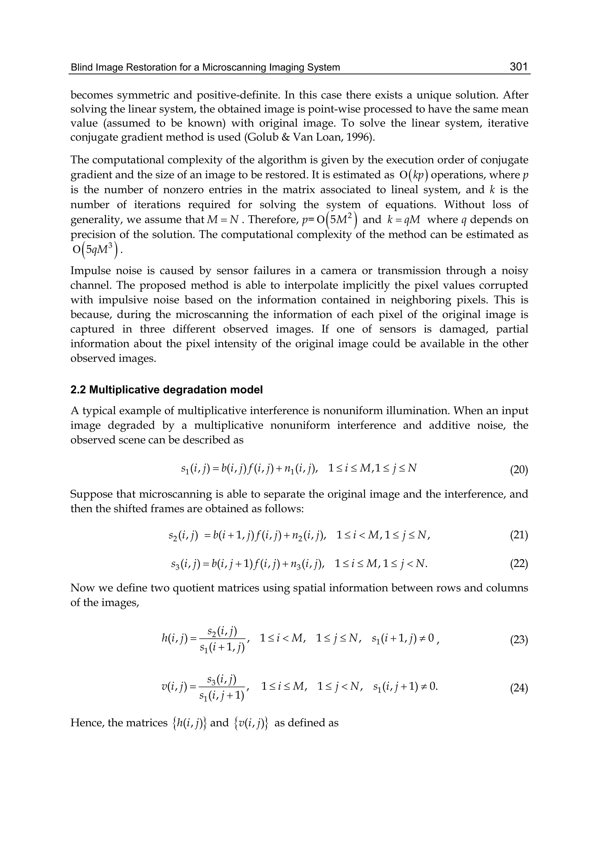
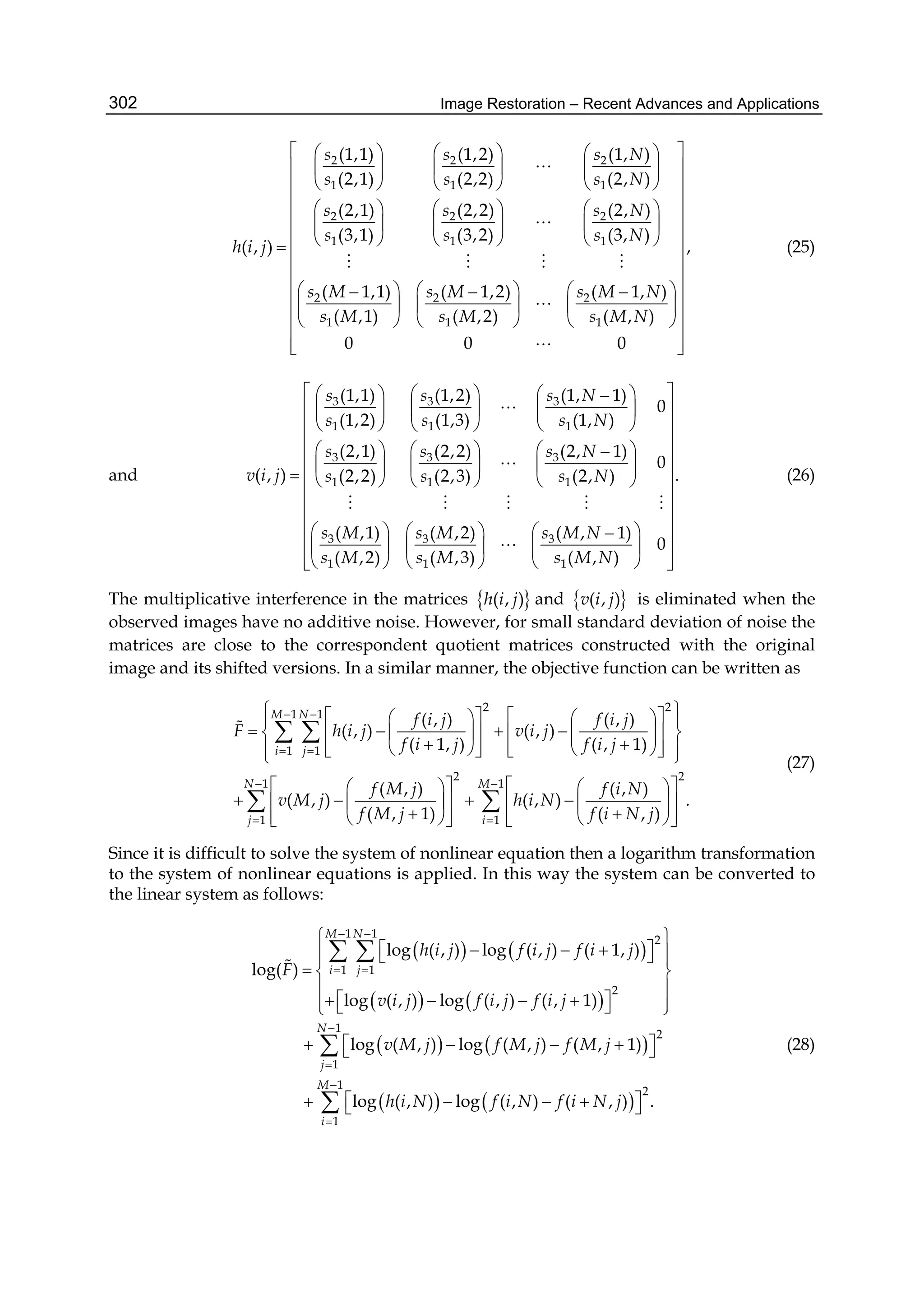
![Blind Image Restoration for a Microscanning Imaging System 303
In a similar manner, the iterative conjugate gradient method can be used for solving this
linear system. Finally, the restored image is obtained by applying the exponential function
to the solution of the linear system. Since this method is based on the conjugate gradient
method, its computational complexity is close to that of for the additive degradation.
Additional expenses are required for logarithm and exponential transformations.
3. Computer simulation results
In this section computer simulation results for restoration of images degraded by additive
and multiplicative interferences are presented. The root mean square error (RMSE) criterion
is used for comparison of quality of restoration. Additionally, a subjective visual criterion is
used. The RMSE is given by
2
( , ) ( , )
, ,
M N
i j
f i j f i j
RMSE f f
MN
(29)
where ( , )f i j is the original image and ( , )f i j is the restored image. The size of images
used in our experiments is 256 256 pixels. The intensity values are in the range of [0,255].
The experiments were performed using a laptop computer (Intel Core 2 Duo 2.26 GHz with
2GB of RAM). To guarantee statistically correct results, 30 statistical trials of each
experiment for different realizations of the random noise process were performed. The
conjugate gradient method is used to solve the linear system. The convergence criterion is
when the residual value drops below 10
10
. The subjective visual criterion is defined as an
enhanced difference between original and restored images. This enhanced difference
(Kober, 2001) is defined as follows:
1 2( , ) ( ( , ) ( , )) ,EDF i j f i j f i j (30)
where 1 and 2 are predetermined constants. In our experiments we set 1 4 and 1 1
for additive and multiplicative models, respectively, and 2 128 . A pixel is displayed as
gray if there is no error between the original image and the restored image. For maximum
error, the pixel is displayed either black or white (with intensity values of 0 and 255,
respectively).
The linear minimum mean square error method is a popular technique in image restoration.
In the case of stationary processes and in the absence of any blur, the method takes a
simplified form of the Wiener smoothing filtering (Jain, 1989). The frequency response of the
empirical Wiener filter is
( , ) ( , )
( , )
( , )
S Noise
Wiener
S
P u v P u v
H u v
P u v
, (31)
where ( , )sP u v is the power spectral density of the observed degraded input scene and
( , )NoiseP u v is the power spectral density of additive interference. It is assumed that all
degradation parameters for the Wiener filter are exactly known. Note that the proposed](https://image.slidesharecdn.com/imagerestorationrecentadvancesandapplications-160714160024/75/Image-restoration-recent_advances_and_applications-313-2048.jpg)
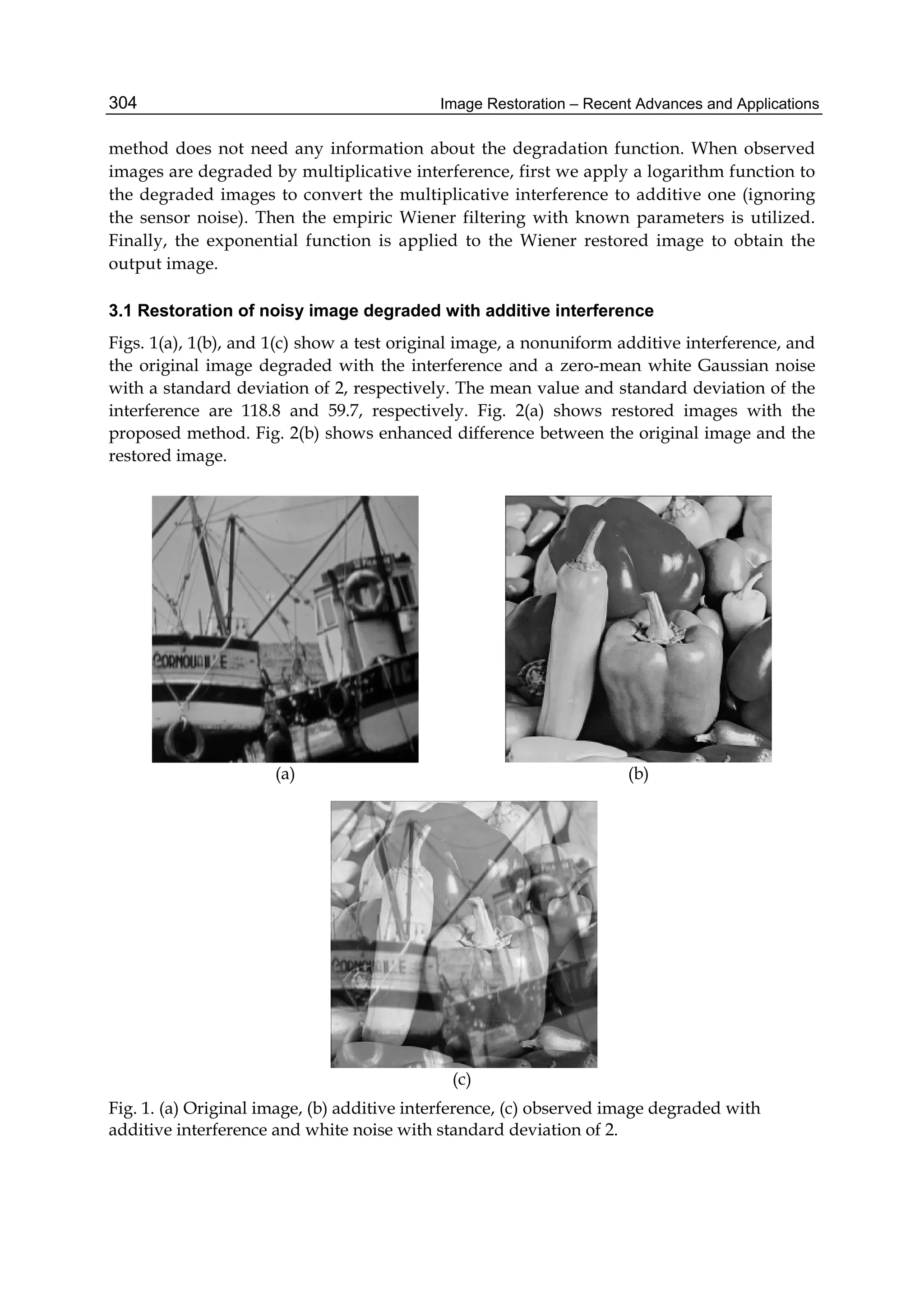
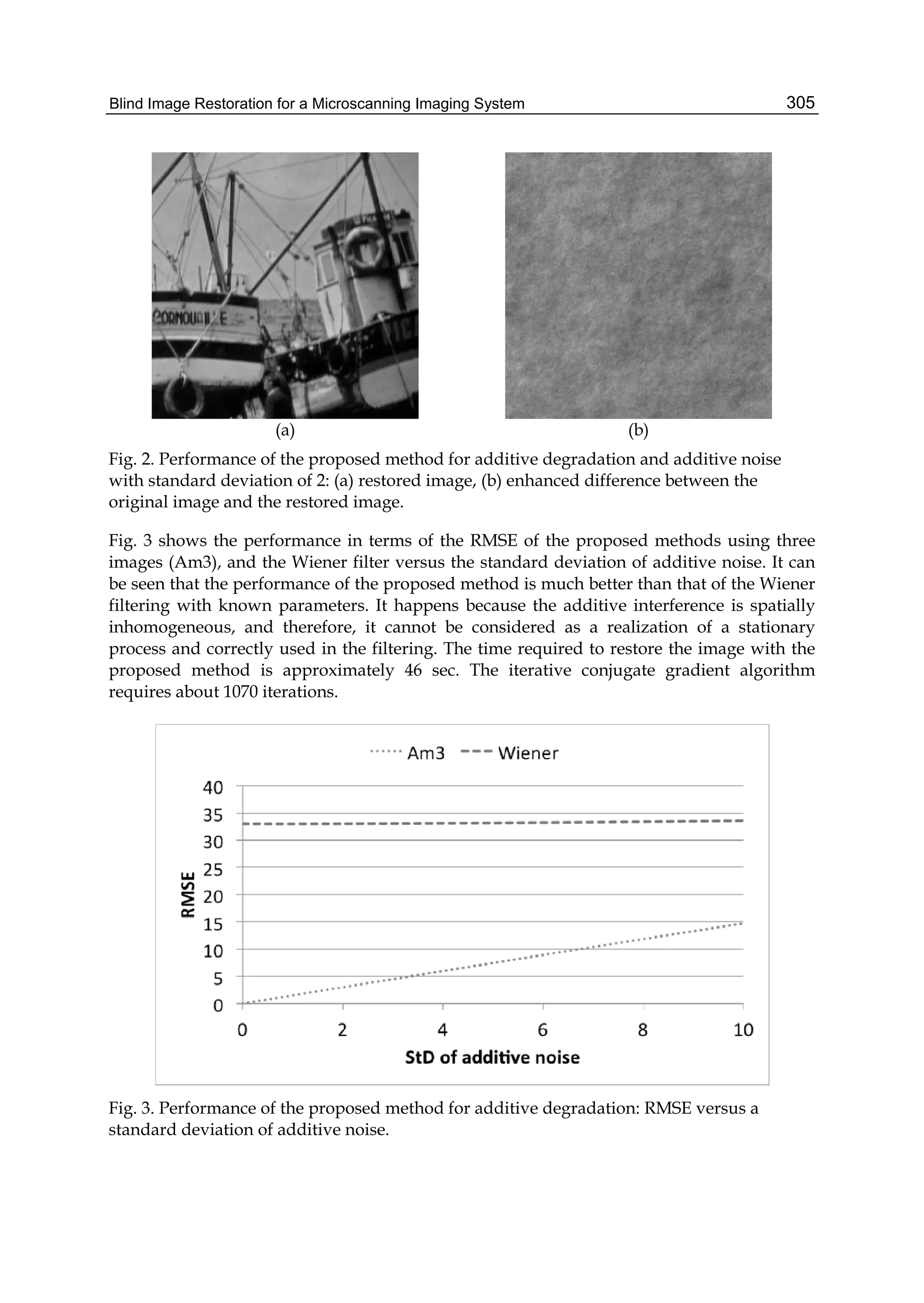
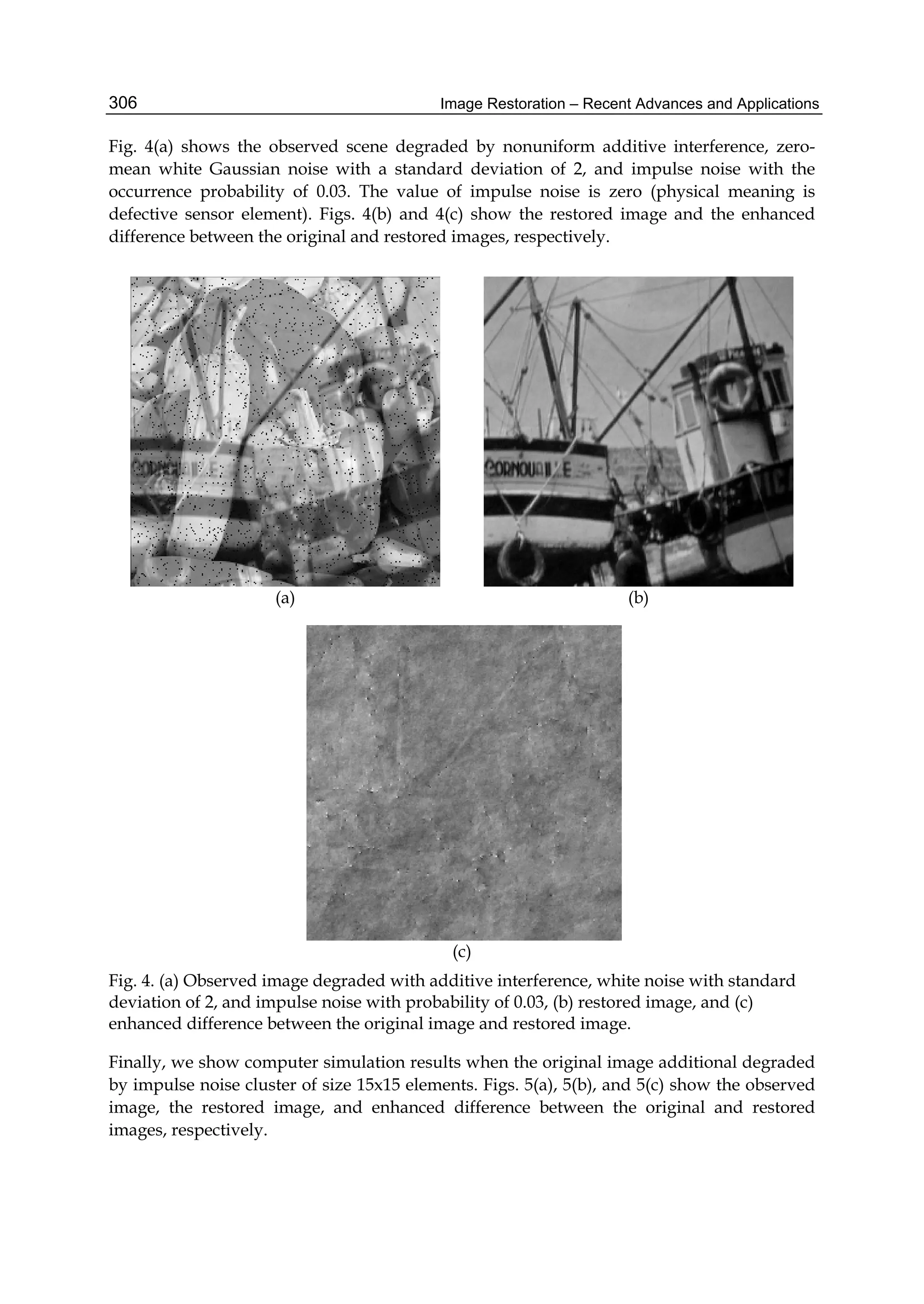
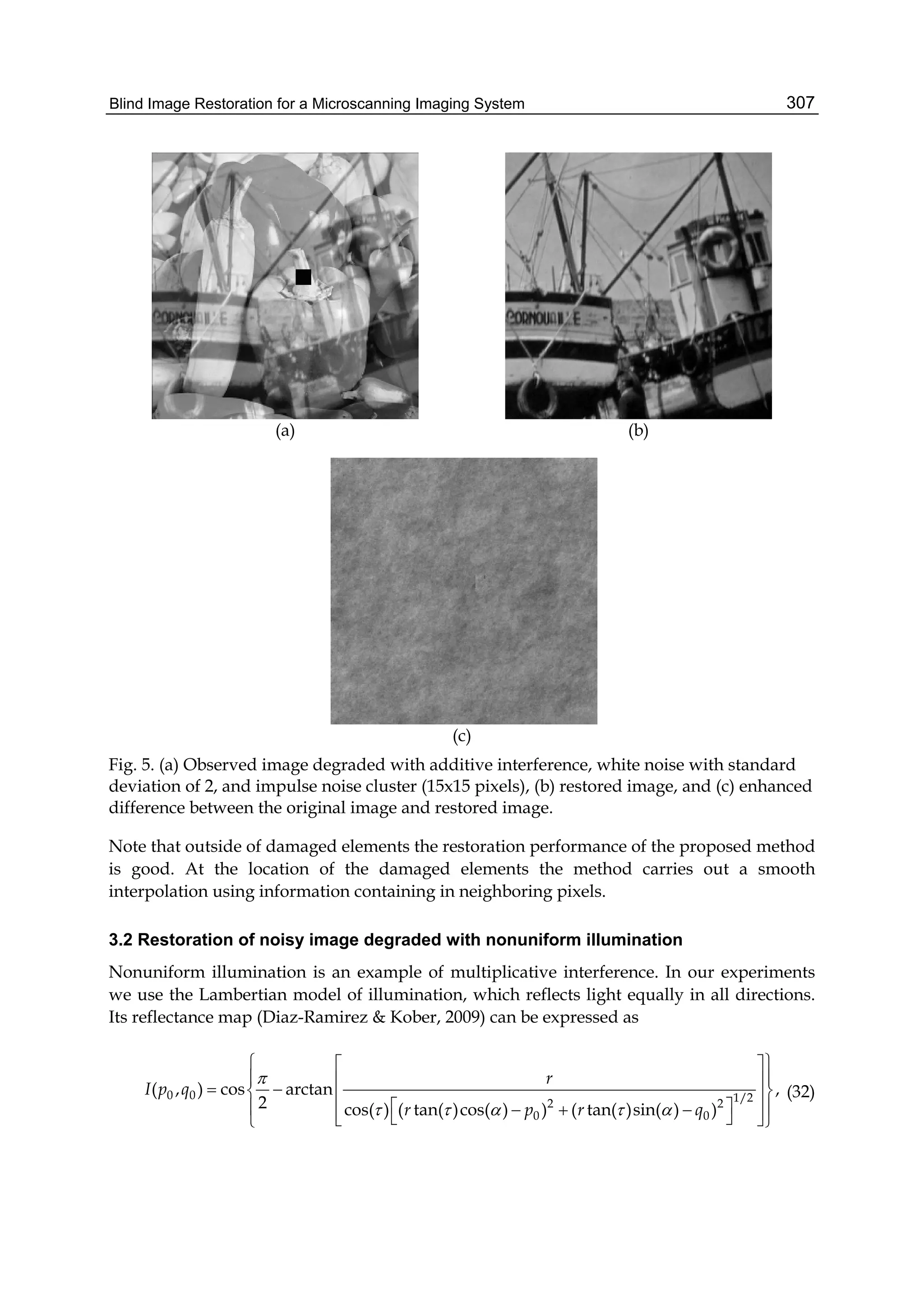
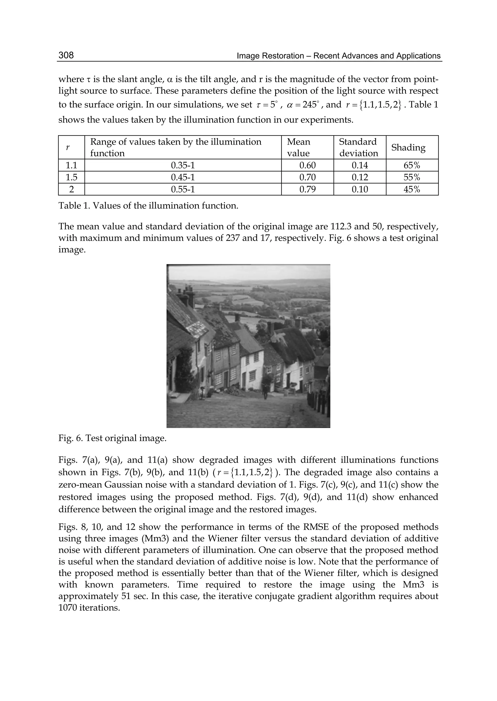
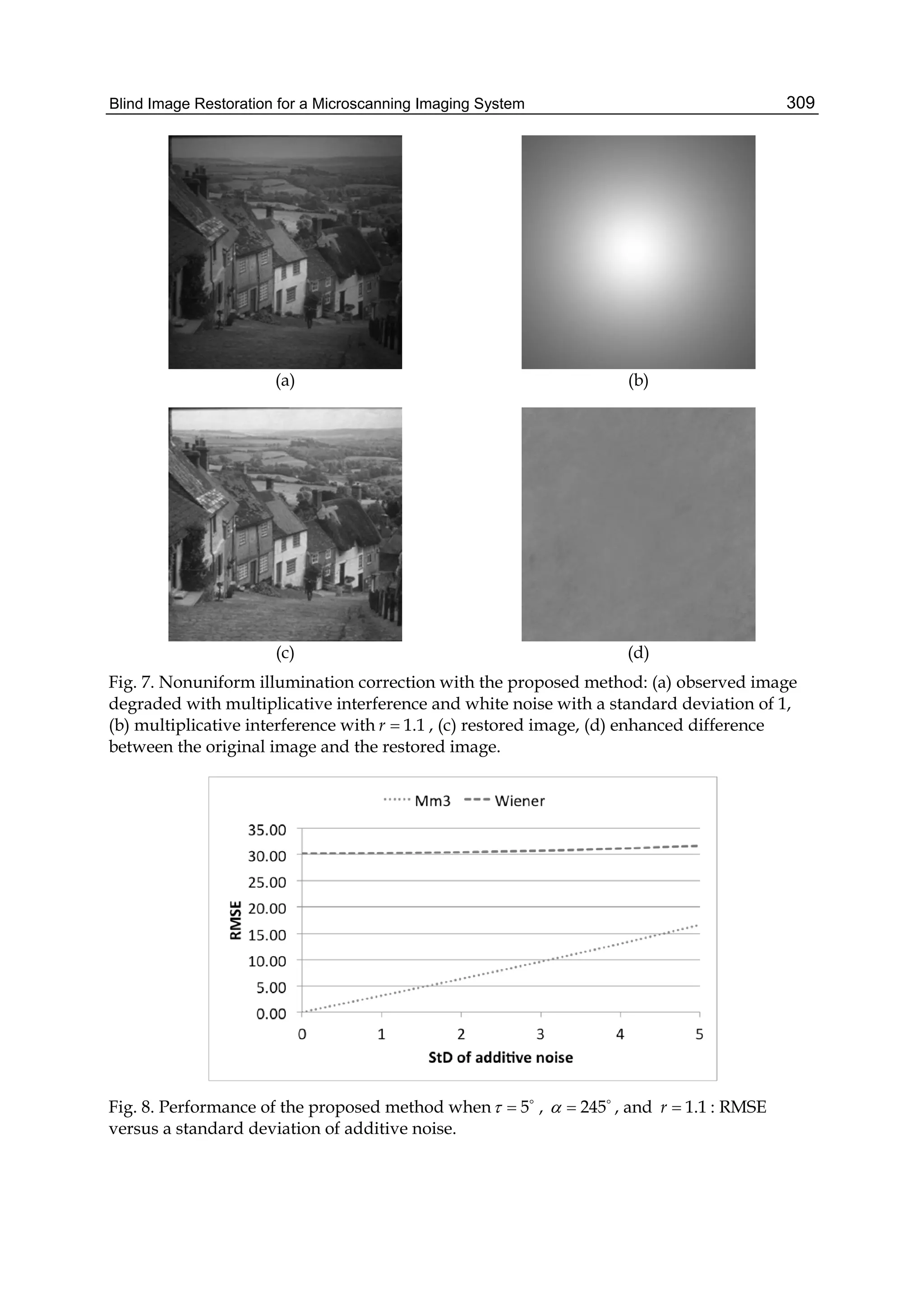
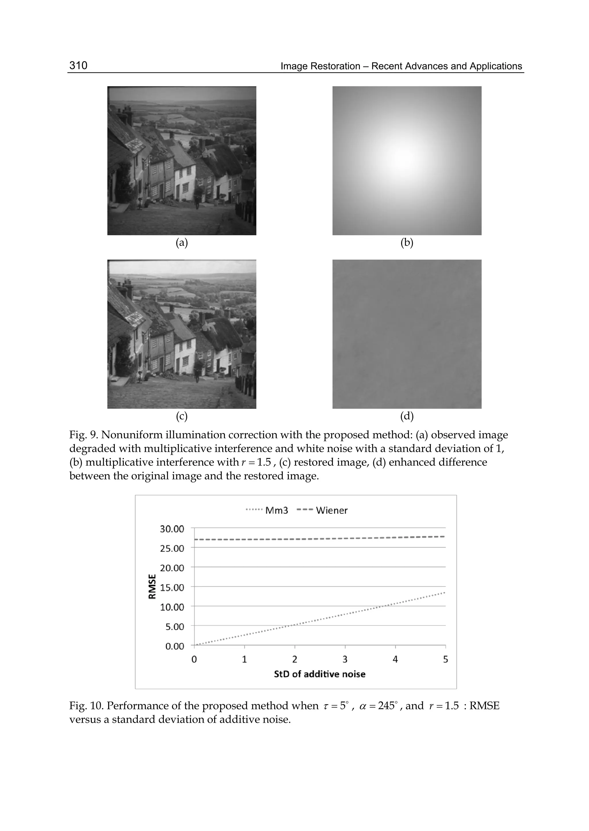
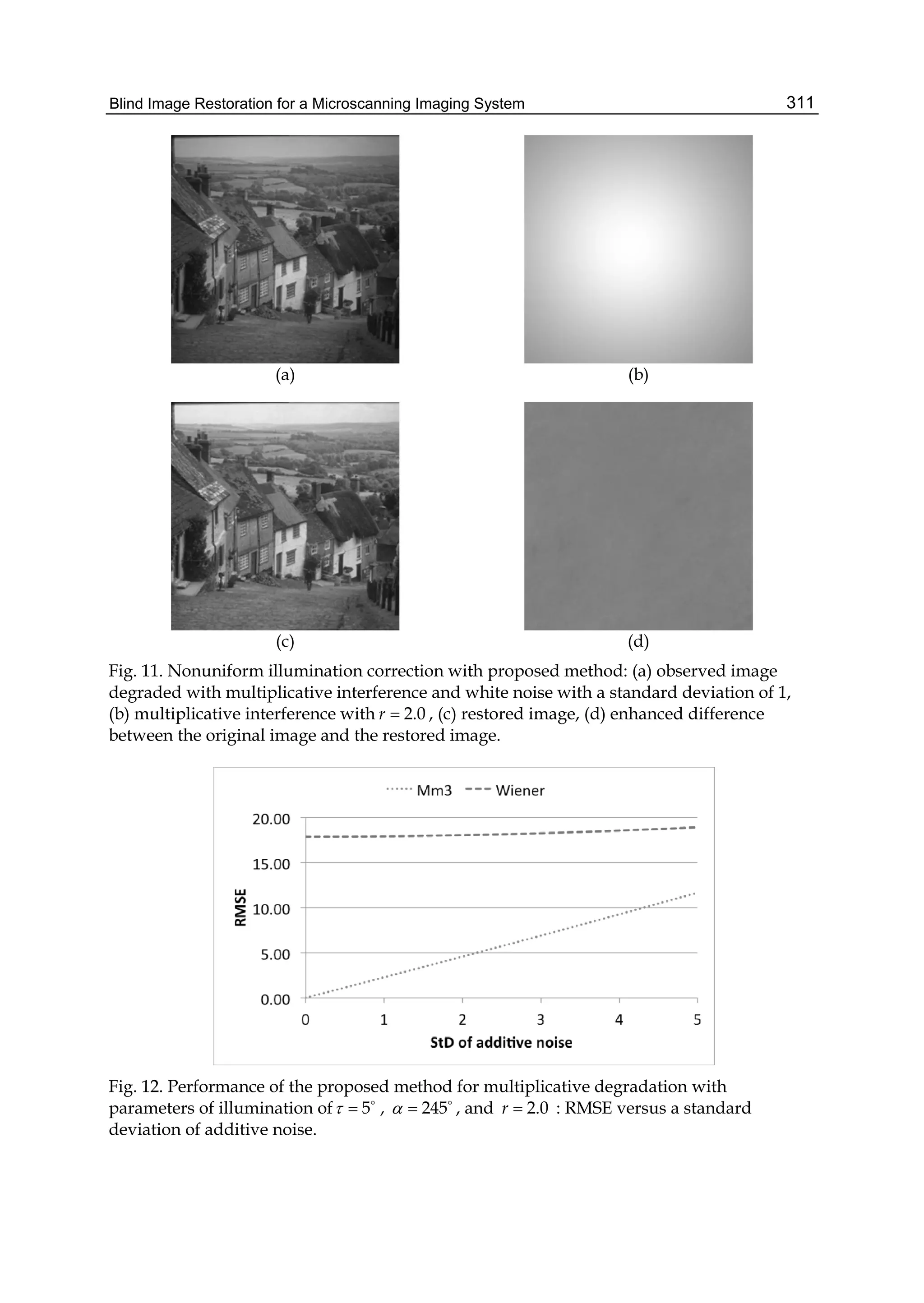
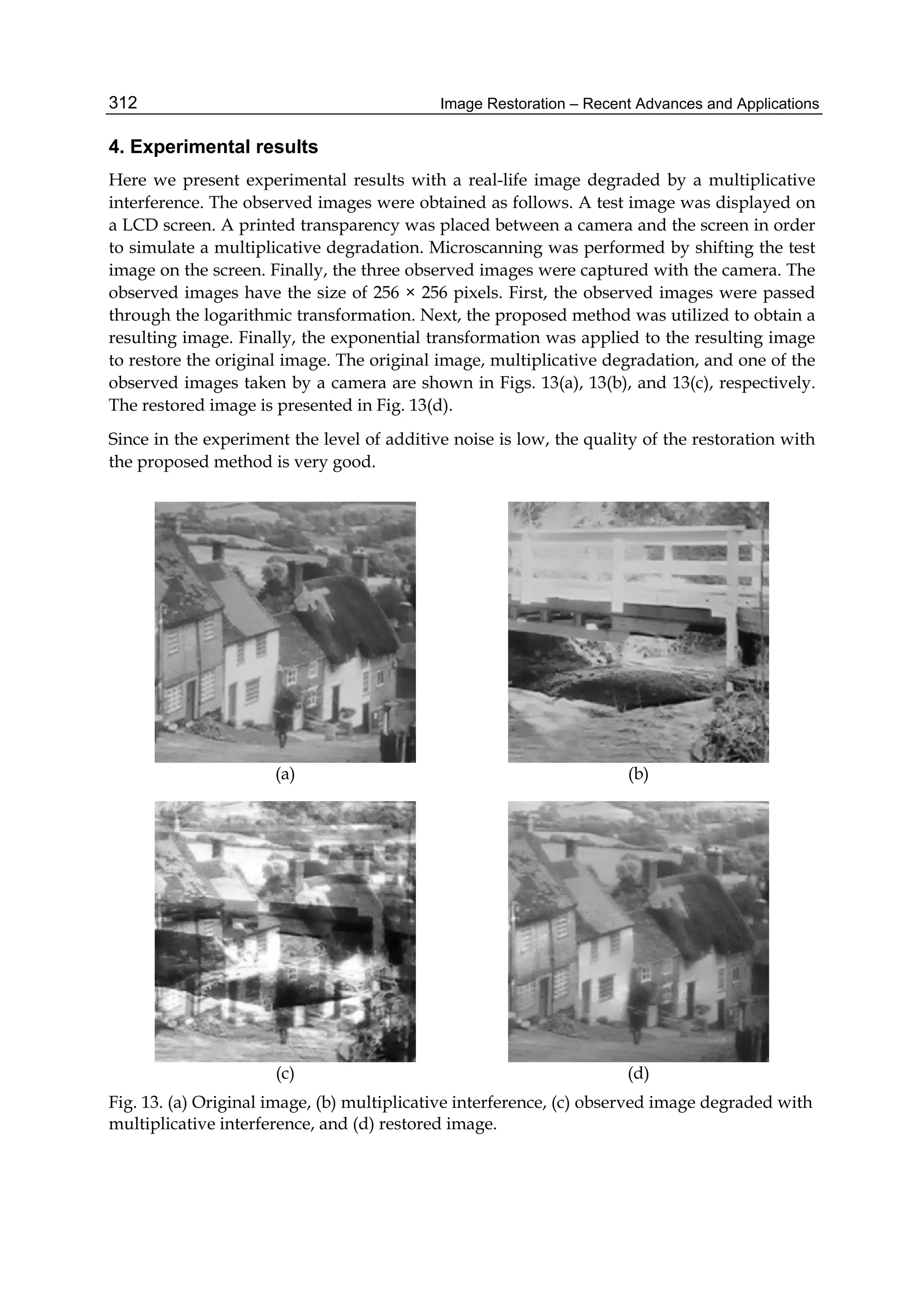
![2 Will-be-set-by-IN-TECH
image. The first section presents the hypothetical model of the time-invariant image blurring
(2D ISI channel). The second one is image capturing section (IECS-ML channel) modeling all
significant noises incident this kind of capturing systems. Such noises rise especially in the
camera sensor with on-chip electronics, but no only there. The last section is the MAP criterion
based iterative detector (restorative circuits) containing IDN with its front-end, so-called soft
output demodulator (SODEM).
Restorative
Photon noise
(Blurring)
channel
2D ISI
˜q(i, j)
circuits
Quantization noise
SO[ ˇd(i, j)]
Thermal noise
Readout noise
(Sensor noises)
d(i, j)
Light rays
(image)
ˆd(i, j)
SI[ ˇd(i, j)]
SO[ˇq(i, j)]
converter
A/D
converter
q → V
SI[ˇq(i, j)]
rd(i,j)
r(i,j)
IECS-ML channel
Restored
picture
DEC
CCD
(CMOS)
Sensor
(FSM)
network
Encoding
SODEM
(FSM−1)
IDN
Fig. 1. Block diagram of a CCD/CMOS camera with dichromatic image restorative section.
3. Deterministic 2D ISI channel (blurring model)
A time-invariant image blurring can be emulated by the signal transmission through the 2D
ISI channel defined via convolution
˜q(i, j) = f (A, Nd(i, j) ⊂ D)
= ∑
0≤i ,j ≤HA,WA
a(i , j )d(i + i , j + j ), (1)
where Nd(i, j) = {d(i + i , j + j )}0≤i ,j ≤HA,WA
denotes the convolution region and D =
[d(i, j)]i,j the page of black and white pixels d(i, j) ∈ {d( )}Md
=1 = {0, 1} (relative photon
quantity impacting at the lens in several par-axial rays). The discrete 2D finite impulse
response A = [a(i , j )]0≤i ,j ≤HA,WA
with the high HA and width WA model time-invariant
image blurring. There we focus closer to the two basic time-invariant distortion — defocusing
in the imperfectly adjusted lens and blurring due to object moving.
3.1 Defocusing in the inperfectly adjusted lens
The image blurring in a defocused lens can be mathematically imitated as the Gaussian
blurring channel (GBC). It is defined by the point spread function PSF(x, y) = Δ
π e−Δ(x2
+y2
),
where Δ is the spread parameter. Two examples of PSF(x, y) with different Δ shows Fig. 2.
If we want transform such PSF to the 2D ISI channel, we have to assume approximation,
that the distribution of light is uniform on the flats with the size and shape congruous to the
316 Image Restoration – Recent Advances and Applications](https://image.slidesharecdn.com/imagerestorationrecentadvancesandapplications-160714160024/75/Image-restoration-recent_advances_and_applications-326-2048.jpg)
![2D Iterative Detection Network Based Image Restoration: Principles, Applications and Performace Analysis 3
sensor cells. Thereafter, the discrete convolution kernel can be got by the integration a(i, j) =
i+1/2
i−1/2
j+1/2
j−1/2
PSF(x, y)dxdy = Δ
4 (erf(i − 1/2) − erf(i + 1/2))(erf(j − 1/2) − erf(j + 1/2)) of the
PSF(x, y) over the individual sensor cells. They are marked in Fig. 2 by the carnation lines
and adjusted, without detriment to generality, as the unit size areas. Concretely, the results of
the mentioned integration in our examples are two kernels
AGBC,3/10 =
⎡
⎣
0.0458 0.1172 0.0458
0.1172 0.3000 0.1172
0.0458 0.1172 0.0458
⎤
⎦ , ASGBC,6/10 =
⎡
⎣
0 0.0872 0
0.0872 0.6000 0.0872
0 0.0872 0
⎤
⎦ , (2)
marked in the given figure by red stem graphs. The first is 9-ray kernel and the second one is
5-ray kernel with suppressed insignificant rays.
(a) AGBC,3/10. (b) ASGBC,6/10.
Fig. 2. The two examples of GBCs with corresponding convolutional kernels.
a(0, 0) = 1a(0, 0) = 0.2 a(0, 0) = 0.3 a(0, 0) = 0.4 a(0, 0) = 0.5 a(0, 0) = 0.7
Fig. 3. Examples of the defocusing by GBC on the QR code snapshot.
3.2 Blurring due to object moving
We have an object moving on the certain known trajectory as well as in Fig. 4. Each point
of this object pass the curve s(t ) = [sx(t ) sy(t )] with the starting ss = s(t) and ending
se = s(t + Te) point. These points are projected through the lens (it is not included to Fig. 4
for simplicity) to the plane {bx, by} of the CCD/CMOS sensor, where Te is the exposure
time. We denote impulse response of the channel emulating blurring due to object moving
as ABOM,α and with respect to discrete character of this response let us approximate the
317
2D Iterative Detection Network Based
Image Restoration: Principles, Applications and Performance Analysis](https://image.slidesharecdn.com/imagerestorationrecentadvancesandapplications-160714160024/75/Image-restoration-recent_advances_and_applications-327-2048.jpg)
![4 Will-be-set-by-IN-TECH
realization of par-axial intensity on the plane {bx, by}, in the time t, as the mosaic D(x, y) =
∑i,j d(i, j)fp(i, j, x, y) of pixels d(i, j) ∈ {d( )}Md
=1 shaped by square function
fp(i, j, x, y) = 1 iff |x − iLp| ≤
Lp
2 ∧ |y − jLp| ≤
Lp
2
0 otherwise
, (3)
where Lp establish their size, that is equal or less then size Lc of the sensor cell (potential well).
Light
rays
Object
Sensor
by
bx
v
t
t + Te
ss
se
Fig. 4. The projection of the moving object point to the CCD/CMOS sensor plane.
On the basis of declared definitions and approximations, we can subsequently express useful
signal impacting the sensor by the convolution Eq. 1 emulating the situation, when the
snapshot D, gained in the time t, is slided on the sensor surface and stepwise trapped to
the its cells. The said fact can be also conceived from the opposite side, when potential well
sliding on the immovable pattern D. If the velocity radial component is insignificant in the
comparison with axial component (expansion of the object is negligible between times t and
t + Te) and starting time t is equated to zero, we can obtain the impulse response coefficients
by the integration
a(i , j ) ∝
Te
0
sy(t )+ 1
2 Lp
sy(t )− 1
2 Lp
sx(t )+ 1
2 Lp
sx(t )− 1
2 Lp
fp(i(ss) + i , j(ss) + j , x , y )dx dy dt . (4)
This situation illustrate Fig. 5a or Fig. 5b. The responses
ABOM,0 = [ 1
12
1
6
1
6
1
6
1
6
1
6
1
12 ]T
, ABOM,π/4 =
⎡
⎢
⎢
⎢
⎢
⎣
1
6
1
12 0
1
12
1
3
1
12
0 1
12
1
6
⎤
⎥
⎥
⎥
⎥
⎦
(5)
can be stated as the examples of such distortion channels that come from Eq. 4 biased by
angles ϕ = 0, ϕ = π
4 and with confinement only to equable movement, when s(t ) is linear
function of time t .
318 Image Restoration – Recent Advances and Applications](https://image.slidesharecdn.com/imagerestorationrecentadvancesandapplications-160714160024/75/Image-restoration-recent_advances_and_applications-328-2048.jpg)
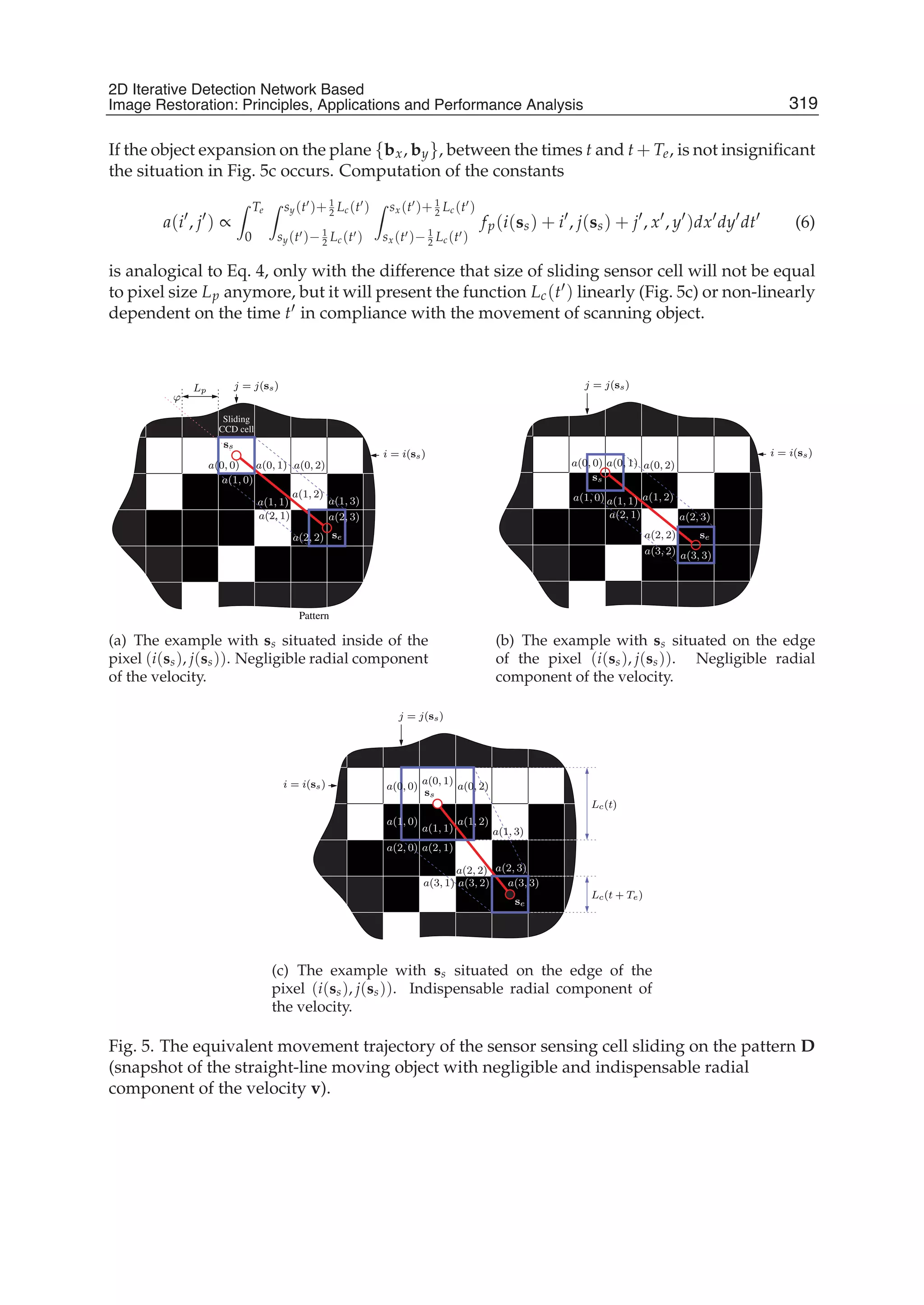
![6 Will-be-set-by-IN-TECH
3.3 Hypothetical cellular model of a 2D ISI channel — Encoding network (EN)
The convolution Eq. 1 can be emulated by certain 2D hypothetical encoding network (EN).
The assembly of this EN is variable and contains specific, relatively simple, functional blocks
fG(). We denote these functional blocks as general processing elements (GPEs) and one such
elements is illustrated in Fig. 6a.
In principle, a GPE presents a simple FSM whose inputs as well as outputs are variables S(k)
discrete in values, that are derivable from alphabets {S( )(k)} . The inputs together with the
outputs consequently create the set N = k S(k) flowing from the alphabet {N ( )} .
/
S(k)
S(K)
S(k + 1)
S(2) S(K − 1)
S(1)
fG( )
(a) A GPE.
SO[ ˇS(k)]
SI[ ˇS(k)]
SI[ ˇS(1)]
SO[ ˇS(1)]
SI[ ˇS(2)]
SO[ ˇS(2)]
SI[ ˇS(k + 1)]
SO[ ˇS(k + 1)]
SI[ ˇS(K − 1)]
SO[ ˇS(K − 1)]
SO[ ˇS(K)]
SI[ ˇS(K)]
f−1
G ( )
(b) A SISO module.
SO[ ˇS(k + 1)]
SI[ ˇS(k + 1)]
SI[ ˇS(K)]
SO[ ˇS(K)]
SO[ ˇS(K − 1)
SI[ ˇS(K − 1)]
SI[ ˇS(1)]
()C() −1
SO[ ˇS(1)]
−1
() C ()
SO[ ˇS(k)]
()C() −1
SI[ ˇS(k)]
() C ()
S[N()]
()C() −1
{S[N()]}
−1
() C ()M
ˇN : ˇS(k)
SI[ ˇS(2)]
SO[ ˇS(2)]
−1
C
ˇS(k)∈ ˇN
(c) Structure of a SISO module.
Fig. 6. A general processing element (GPE) and its soft inversion (SISO module).
4. Random IECS-ML channel (noise model)
4.1 Composite noise of the CCD/CMOS sensor
The presence of the signal independent composite CCD/CMOS sensor noise in mutually
correlated rays 0 ≤ ˜q(i, j) ≤ 1 can be expressed as the blurred image transmission through
320 Image Restoration – Recent Advances and Applications](https://image.slidesharecdn.com/imagerestorationrecentadvancesandapplications-160714160024/75/Image-restoration-recent_advances_and_applications-330-2048.jpg)
![2D Iterative Detection Network Based Image Restoration: Principles, Applications and Performace Analysis 7
the random IECS-ML channel with I/O equation r(i, j) = C ˜q(i, j) + wT(i, j) + wR(i, j), where
r(i, j) is the channel output, wT(i, j) is the total thermal noise accumulated with the useful
signal q(i, j) = C ˜q(i, j) as a charge in the CCD sensor cell at the position (i, j) and wR(i, j)
is the readout noise. The constant C (above limited by a full well capacity FWC of the CCD
sensor) defines a quantity of generated charge and it is directly proportional to the exposure
time Te.
4.2 Quantization noise of the A/D converter
The output r(i, j) (IECS-ML channel output also registrable in the matrix form R = Q +
WT + WR for entire sensor) is further quantized in the Nb-bit A/D converter that can be
approximated by the random channel rd(i, j) = r(i, j) + wQ(i, j) with uniformly distributed
noise wQ(i, j) in light of probability theory. We denote the output of this converter as
rd(i, j) = Q(r(i, j)), where Q(ξ) = ∑1≤ ≤2Nb H(ξ − tQ( )) and H(ξ) = {0
1
iff ξ<0
otherwise is a
Heaviside step function. For simplicity we will assume the linear quantization only with
threshold values
tQ( ) =
0
( − 1)ΔQ + 1/2
iff
iff
= 1
1 < ≤ 2Nb
(7)
and quantization step ΔQ, where for the highest quantization level tQ(2Nb ) ≤ FWC is applied.
5. Image restoration — Symbol and page 2D MAP detection
5.1 Optimal MAP detection
The channel has independent eliminated states (IECS), if noise sources in CCD sensor cells are
mutually independent. It makes joint probability density function (PDF) pW(Ξ) = ∏i,j pw(ξ)
as the product of marginal densities. The channel is memory-less (ML), if the current x(i, j)
depends only on the corresponding q(i, j). The fulfillment of both conditions creates the
likeli-hood function
pR(Ξ| ˇQ) =
W
pR|Q,W(Ξ| ˇQ, Ξ )pW(Ξ )dΞ
= ∏
i,j
w(i,j)
pr|q,w(ξ| ˇq(i, j), ξ )pw(ξ )dξ
pr(ξ| ˇq(i,j))
(8)
factorizable that is necessary to transition from a single-stage detector to an IDN.
The optimal 2D MAP detector is based on the criterion
ˆd(i, j) = arg M
ˇd(i,j)
M
ˇD: ˇd(i,j)
S[Rd, ˇD] , (9)
where ˆd(i, j) denotes the wanted estimation, ˇd(i, j) denotes a testing estimator (takes
individual values from data alphabet), ˇD : ˇd(i, j) denotes the set of possible image realizations
containing the estimator ˇd(i, j) and M with M denote certain types of marginalization
operators.
321
2D Iterative Detection Network Based
Image Restoration: Principles, Applications and Performance Analysis](https://image.slidesharecdn.com/imagerestorationrecentadvancesandapplications-160714160024/75/Image-restoration-recent_advances_and_applications-331-2048.jpg)
![8 Will-be-set-by-IN-TECH
The quantity S[Rd, ˇD] is to be understood as some kind of the joint soft measure and due to
IECS-ML condition fulfillment
S[Rd| ˇD] = C
i,j
S[rd(i, j)| ˇD]
= C
i,j
S[rd(i, j)| ˇNd(i, j) ⊂ ˇD] (10)
with assumption of a statistically independent data S[ ˇD] = C
i,j
S[ ˇd(i, j)] can be decomposed to
the form
S[Rd, ˇD] = S[Rd| ˇD] C S[ ˇD]
= C
i,j
S[rd(i, j)| ˇNd(i, j) ⊂ ˇD] C C
i,j
S[ ˇd(i, j)] (11)
that is joined by certain types of combination operators ( C , C ). On the basis of
marginalization and combination operators, we can split detectors into four groups in light
of detection technique (symbol or page) and implementing domain (probability P[ ] or
equivalent logarithmic metric M[ ] = − ln(P[ ])). All possibilities are summarized in Table 1.
The symbol technique (SyD) seeks to minimize of the actual symbol detection error only.
The page detection (PgD) has tendency to minimization the entire page detection error.
The most numerically effective is the Md-PgD alternative, because it contains the simple
combination operator as well as the simple marginalization operator. Close to the Md-PgD,
the Md-SyD conjunction with the relatively simple marginalization operator min∗(x, y) =
min(x, y) − ln(1 + e−|x−y|).
Domain S[ ] Detection M M C C C −1
Probability (Pd) P[ ] Page (PgD) max max Π × ÷
Probability (Pd) P[ ] Symbol (SyD) max Σ Π × ÷
Metric (Md) M[ ] Page (PgD) min min Σ + −
Metric (Md) M[ ] Symbol (SyD) min min∗ Σ + −
Table 1. Summary of combination and marginalization operators.
5.2 Suboptimal MAP detection
The direct evaluation of the ˆD from the criterion (9) (single-stage detection) is impossible,
because it requires a sequent substitution of all potential image realizations ˇD. But Eq. 10
(IECS-ML condition) makes possible decomposition of the detection problem from the entire
page D to the level of individual (mutually overlapping) convolution regions Nd(i, j),
corresponding to individual captured pixels. Therefore, we can substitute the single-stage
MAP detector by the sub-optimal iterative detection network (IDN).
Such network is formed from a definite number of functional blocks, so-called soft inversions
(SISO modules), that exchange the soft measures with each other. The SISO modules present
statistical devices complementary to the GPEs in the appropriately designed hypothetical EN
322 Image Restoration – Recent Advances and Applications](https://image.slidesharecdn.com/imagerestorationrecentadvancesandapplications-160714160024/75/Image-restoration-recent_advances_and_applications-332-2048.jpg)
![2D Iterative Detection Network Based Image Restoration: Principles, Applications and Performace Analysis 9
emulating the image blurring. The fulfillment of the condition IECS-ML enables a usage of
such GPEs that compose the hypothetical realization ˇD of a sensing image even by smallest
parts (by individual pixels ˇd(i, j)) if this yields a implementation benefits in light of concrete
modeled distortion.
The IDN output can be regarded as a optimal (identical with the output of single-stage
detector) after the execution of infinite number of iterations (information interchange between
inversions). It is not practicable. Therefore, the IDN with the finite number of iterations
is sub-optimal detector, that generally provides an inferior estimation to the single-stage
detector. Roughly speaking the IDN contains simpler SISO modules, the IDN is more
numerically effective and more sub-optimal (it includes more iteratively refining variables).
In the course of each iteration I of the IDN, from count NI, is every SISO module once
activated at the least. The activation rests in the reading of soft measures (whole probability
or metric densities {SI[S( )(k)]} , corresponding to certain random variable S(k) in the
hypothetical model) on inputs of a SISO module, followed by the enumeration of output soft
measures (whole densities {SO[S( )(k)]} ). The current iteration concludes the exchange of
soft measures
{SO[S( )(k)]}
{SI[S( )(k)]}
→
←
{SI[S( )(k)]}
{SO[S( )(k)]}
(12)
among the neighboring modules. After execution of all iteration NI, the estimations of all
wanted (output) random variables are performed from the formula
ˆS(k) = arg M
ˇS(k)
[SI[ ˇS(k)] C SO[ ˇS(k)]]. (13)
We express this operation as a hard decision provided by a decision block (DEC).
6. Iterative detection networks
6.1 IDN topology and soft inversion f −1
G () (SISO module) of general processing element
fG() (FSM)
An IDN presents a soft inversion of an arbitrary EN formed from certain mutually
concatenated GPEs that jointly execute an arbitrary processing with input signal. In the our
case, as was said in the paragraph 3.3, such EN executes the convolution Eq. 1 and due to
fulfillment of the IECS-ML condition can contain the simplest GPEs working on the level
of individual pixels. The IDN topology exactly agrees to the EN topology only with the
difference, that each of GPE is substituted by its SISO module, just like in Fig. 6a, 6b. The
signal processing in the soft inversion is implied in Fig. 6c and takes place in two steps. Firstly,
the inputs {SI[S( )(k)]} ,k are combined to particular joint soft measures
S[ ˇN ] = C
ˇS(k)∈ ˇN
SI[ ˇS(k)] for ∀ ˇN . (14)
Consequently, all joint measures {S[N ( )]} , corresponding to the set ∀ ˇN of possible
realizations N ( ), are marginalized to outputs {SO[S( )(k)]} ,k
SO[ ˇS(k)] = M
ˇN : ˇS(k)
S[ ˇN ] C −1
SI[ ˇS(k)] for ∀ ˇS(k) (15)
323
2D Iterative Detection Network Based
Image Restoration: Principles, Applications and Performance Analysis](https://image.slidesharecdn.com/imagerestorationrecentadvancesandapplications-160714160024/75/Image-restoration-recent_advances_and_applications-333-2048.jpg)
![10 Will-be-set-by-IN-TECH
that are connected to the inputs {SI[S( )(k)]} ,k of neighboring soft inversions. This update of
soft information is known as a soft inversion activation. The activation accomplishment of all
soft inversions in the IDN afterwards makes one iteration of the IDN.
6.2 Soft-output demodulator
The IDN closely cooperates with the SODEM (Soft output demodulator) providing
fundamental hypothesis about captured signal Rd. This functional block presents a gateway
between the domain of a real realizations (realizations of certain random variables), where are
operated with scalars (factual realizations), and the probability (metric) domain of the IDN,
where are operated with whole densities. The SODEM includes the likeli-hood function (or
transfer function) of the IECS-ML channel emulating all noises incident in the image capturing
system chain (in the our case it is CCD/CMOS camera). The SODEM input forms realization
rd(i, j) that is inside transformed to the discrete a posteriori density {SI[q( )(i, j)]} presenting
the input (sufficient statistic) of the IDN.
Before the sufficient statistic derivation as such, it should be noted that the derivation is purely
theoretical and does not correspond to any particular type of CCD / CMOS sensor. We start
the SODEM derivation with the definition of discrete cut off Gaussian PDF
pN FWC
0
(ξ, μ, σ) ≈
1
√
2πσ
FWC
∑
=0
δ(ξ − ) exp −
( − μ)2
2σ2
+
1
2
δ(ξ − FWC)erfc
2FWC + 1 − 2μ
√
8σ
+δ(ξ) 1 −
1
2
erfc −
1 + 2μ
√
8σ
. (16)
All parameters FWC, ξ, μ, σ, etc. in all densities, we will assume in terms of number of
electrons [-] either directly or as equivalent quantities related to number of electrons (for
example: the quantization noise occurring in the A/D converter, we will consider as if
the equivalent electron noise source deteriorative in the sensor, etc.). On the basis of the
mentioned definition can be formed thermal and readout noise PDFs as
pwT (ξ) ≈
⎧
⎪⎪⎨
⎪⎪⎩
0 iff μT <40
ξ≥70
e−μT
∑ ∈N0
μT
! δ(ξ − ) iff μT <40
ξ<70
pN FWC
0
(ξ, μT,
√
μT) iff μT ≥ 40
(17)
and
pwR (ξ) = pN FWC
0
(ξ, μR, σR). (18)
Both noises together then create the composite noise w(i, j) = wT(i, j) + wR(i, j) and examples
of theirs densities, for certain parameters μT, μR and σR, is shown in Fig. 7.
The mentioned PDFs are biased by three parameters μR, σR and μT. First two parameters are
known, because depend on the sensor readout rate that is also known. The last one is the
nuisance unknown parameter consisting in the unknown CCD/CMOS sensor temperature
and has to be estimated by a suitable way. A ML estimation ˆμ = N−1
∑K
k=1 w(k) can be used
324 Image Restoration – Recent Advances and Applications](https://image.slidesharecdn.com/imagerestorationrecentadvancesandapplications-160714160024/75/Image-restoration-recent_advances_and_applications-334-2048.jpg)
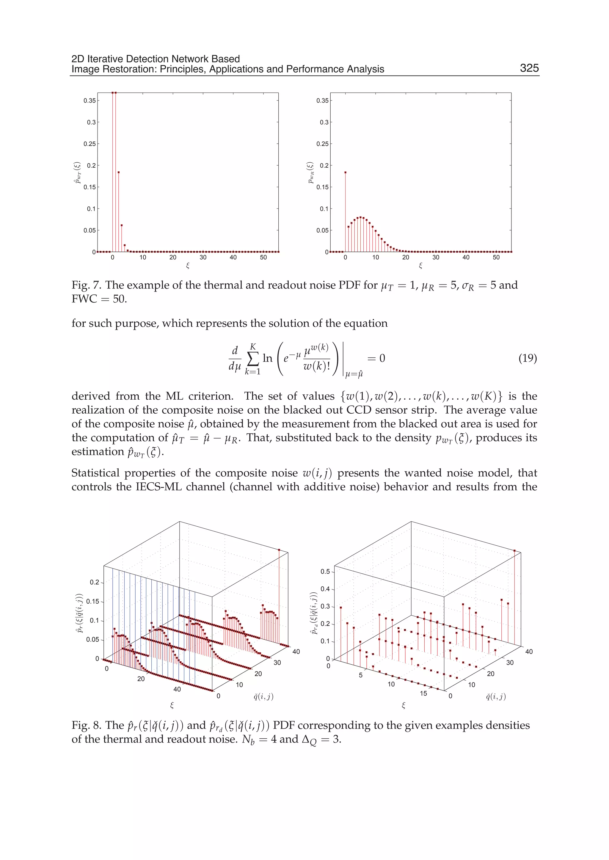
![12 Will-be-set-by-IN-TECH
cut off PDF
ˆpw(ξ) ≈ ˆpw(ξ) + δ(ξ − FWC) 1 −
FWC+ 1
2
− 1
2
ˆpw(ξ )dξ , (20)
based on the convolution
ˆpw(ξ) =
FWC
∑
=0
δ(ξ − )
ξ+ 1
2
− 1
2
ˆpwT ( − ξ )pwR (ξ )dξ (21)
of densities ˆpwT (ξ) and pwT (ξ).
The procedure obtaining the metric SI[ ˇq(i, j)] from the derived noise model begins with the
elimination Eq. 10 of the noise density ˆpw(ξ) out of the likeli-hood function of a channel with
additive noise pR|Q,W(Ξ| ˇQ, Ξ ) = δ(Ξ − ( ˇQ + Ξ )) or pr|q,w(ξ| ˇq(i, j), ξ ) = δ(ξ − ( ˇq(i, j) + ξ )),
assuming perfect knowledge of the noise realization W. The result of this elimination is the
density ˆpr(ξ| ˇq(i, j)) = ˆpw( ˇq(i, j) − ξ). Along with the thermal noise, another source of noise is
found in the chain. It is the quantization noise with the uniform PDF pwQ which is added to
the signal in the A/D converter. It can be eliminated out of the density ˆpr by the integrating
ˆprd
(ξ| ˇq(i, j)) = δ(ξ − 2Nb ) lim
→0+
FWC+ 1
2
tQ(2Nb )−
ˆpr(ξ | ˇq(i, j))dξ
+
2Nb −1
∑
=1
δ(ξ − ) lim
→0+
tQ( +1)−
tQ( )−
ˆpr(ξ | ˇq(i, j))dξ (22)
over individual quantization steps (by averaging with the density pwQ ) of the size ΔQ
expressed in the number of electrons and defined, in our case, by Eq. 7. In Fig. 8 you
can see the examples of the densities ˆpr(ξ| ˇq(i, j)) and ˆprd
(ξ| ˇq(i, j)) coming out of the given
demonstrations in Fig. 7 if and only if ˇq(i, j) ∈ {q( )}
Mq
=1 = {0, 10, 20, 30, 40}. We would like
to emphasize that it is just a simple example and actually the cardinality of set {q( )}
Mq
=1 =
f (A, {Nd(i, j)}
MNd
=1 ) is much larger then 5. Blue lines on Fig. 8 represent boundaries of the
individual quantization steps.
The SODEM output can be obtained from the derived density by the integration
PI[ ˇq(i, j)] =
rd(i,j)+ 1
2
rd(i,j)− 1
2
ˆprd
(ξ | ˇq(i, j))dξ . (23)
On the following Fig. 9a, 9c, 9e, 9g are introduced four examples of the SODEM transfer
function constituting the derived composite CCD/CMOS noise model for the blurring
channel AGBC,3/10 (Eq. 2) and ABOM,π/4 (Eq. 5). For the purpose of higher lucidity was
chosen continuous plotting, although the transfer functions have a discrete domain of
definition. The individual demonstrations of transfer functions afterwards construe with
samples (realizations) of captured images on Fig. 9b, 9d, 9f, 9h.
326 Image Restoration – Recent Advances and Applications](https://image.slidesharecdn.com/imagerestorationrecentadvancesandapplications-160714160024/75/Image-restoration-recent_advances_and_applications-336-2048.jpg)
![2D Iterative Detection Network Based Image Restoration: Principles, Applications and Performace Analysis 13
7. Distributed iterative detection networks
7.1 Distributed IDN marginalizing at the symbol block level
Firstly we focus on the IDNs marginalizing at the symbol block level with horizontal and
vertical state variable. These IDNs result from the EN [1] in Fig. 10a where each node (GPE),
shown in Fig. 11b, creates a one functional block with the fixed system of inputs and outputs
Nf (i, j) = {R(i, j), C(i, j), d(i + HA, j + WA), R(i, j + 1), C(i + 1, j), q(i, j)}, where R(i, j) and
C(i, j) present auxiliary state variables containing more symbols together. Shapes of these
variables are established by the condition
Nd(i, j) R(i, j) ∪ C(i, j) ∪ d(i + HA, j + WA)
⊃ R(i, j + 1), C(i + 1, j). (24)
The optimal decomposition of the convolution region is Nd(i, j) = R(i, j) ∪ C(i, j) ∪ d(i +
HA, j + WA) and it is possible when a(HA, WA) = 0.
In the case of a channel AGBC,a(0,0), with regard to the condition Eq. 24, the variables are
R(i, j) = {d(i, j), d(i, j + 1), d(i + 1, j), d(i + 1, j + 1), d(i + 2, j), d(i + 2, j + 1)} and C(i, j) =
{d(i, j), d(i, j + 1), d(i, j + 2), d(i + 1, j), d(i + 1, j + 1), d(i + 1, j + 2)}. Their shapes you can see
in Fig. 12a. In a similar way we can get decomposition of the Nd(i, j) for a channel AGBC,a(0,0).
One of possible results is shown in Fig. 12b.
The IDN has same topology as the EN and each its node forms SISO module, illustrated in
Fig. 11b, performing the combination
S[ ˇNf (i, j)] = SI[ ˇR(i, j)] C SI[ ˇC(i, j)] C SI[ ˇd(i + HA, j + WA)] C SI[ ˇR(i, j + 1)]
C SI[ ˇC(i + 1, j)] C SI[ ˇq(i, j)] (25)
with marginalizations
SO[ ˇR(i, j + j )] = M
ˇNf (i,j): ˇR(i,j+j )
S[ ˇNf ()(i, j)] C −1
SI[ ˇR(i, j + j )] for j ∈ {0, 1}, (26)
SO[ ˇC(i + i , j)] = M
ˇNf (i,j): ˇC(i+i ,j)
S[ ˇNf ()(i, j)] C −1
SI[ ˇC(i + i , j)] for i ∈ {0, 1}, (27)
SO[ ˇd(i + HA, j + WA)] = M
ˇNf (i,j): ˇd(i+HA,j+WA)
S[ ˇNf ()(i, j)] C −1
SI[ ˇd(i + HA, j + WA)], (28)
and
SO[ ˇq(i, j)] = M
ˇNf (i,j): ˇq(i,j)
S[ ˇNf ()(i, j)] C −1
SI[ ˇq(i, j)]. (29)
One iteration of such IDN rests in the serial activation of each SISO module from the upper
left corner to the lower right corner in the IDN as is marked by the light blue curve in Fig. 10a.
After finishing all iterations, of the chosen count NI, the IDN makes hard decisions ˆd(i, j) per
Eq. 13.
327
2D Iterative Detection Network Based
Image Restoration: Principles, Applications and Performance Analysis](https://image.slidesharecdn.com/imagerestorationrecentadvancesandapplications-160714160024/75/Image-restoration-recent_advances_and_applications-337-2048.jpg)
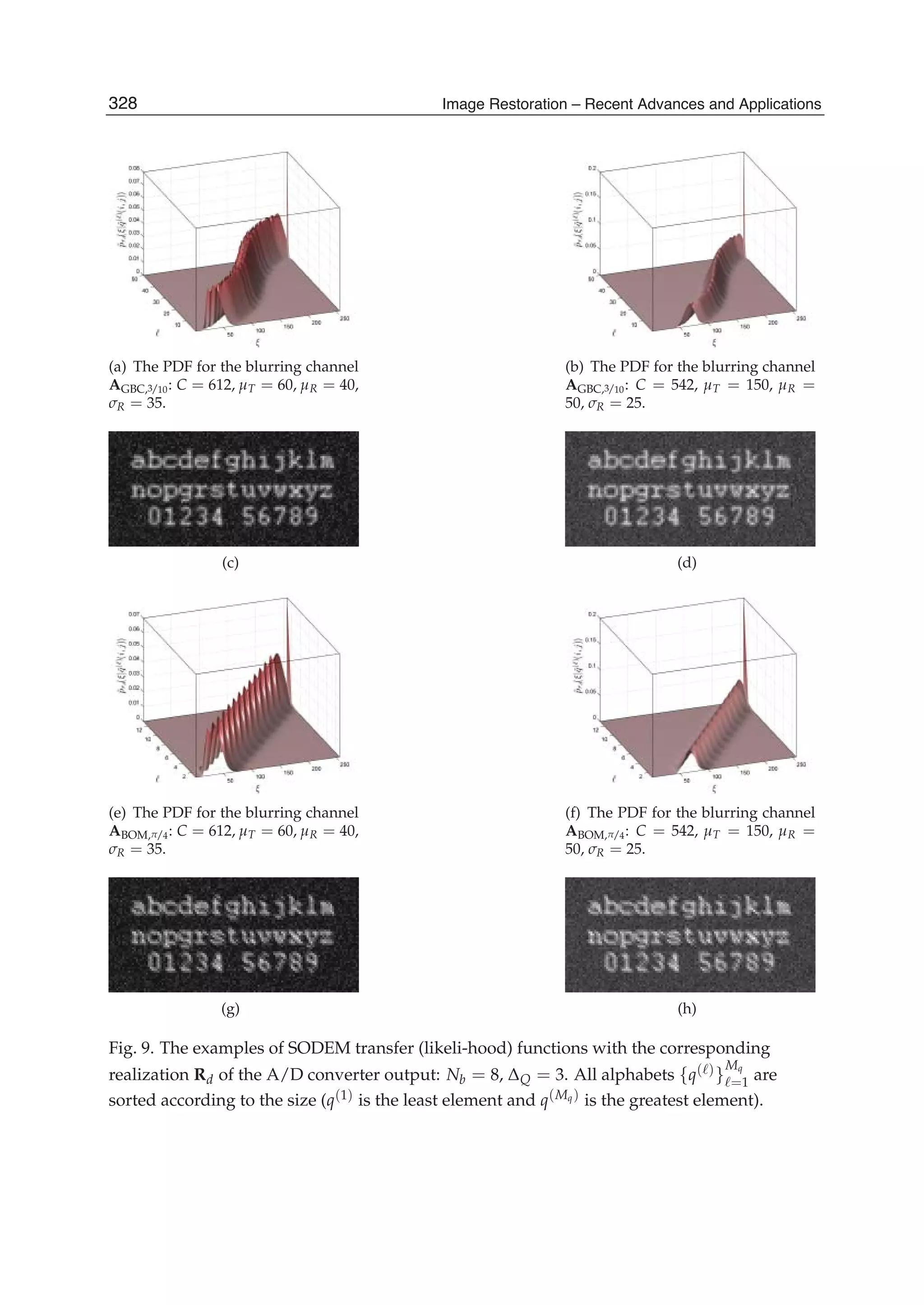
![2D Iterative Detection Network Based Image Restoration: Principles, Applications and Performace Analysis 15
SI[ˇC(i+1,j)]SO[ˇC(i+1,j)]
SI[ ˇR(i, j + 1)]
SO[ ˇR(i, j + 1)]
SO[ ˇR(i, j + 1)]
SI[ ˇR(i, j + 1)]
i + 2
i + 1
i
j + 2
R(i, j + 1)
schedule
Activation
j + 1j
EN
EN
C(i+1,j)
IDN
SO[ˇC(i+1,j)]SI[ˇC(i+1,j)]
IDN
(a) The EN and IDN marginalizing at the symbol
block level.
i + 2
i + 1
i
j + 2
schedule
Activation
j + 1j
(b) The EN and IDN marginalizing at the symbol
block level with bias state variables.
Fig. 10. The topology of the EN and IDN with denotation of the IDN activation schedule.
R(i, j)
C(i, j)
C(i + 1, j)
q(i, j)
R(i, j + 1)
d(i + HA, j + WA)
f( )
(a) The EN cell.
SO[ ˇd(i + HA, j + WA)]
SI[ ˇd(i + HA, j + WA)]
SO[ ˇR(i, j + 1)]
SI[ ˇR(i, j + 1)]
SI[ ˇR(i, j)]
SO[ ˇR(i, j)]
SI[ˇq(i, j)]
SO[ˇq(i, j)]
SO[ˇC(i,j)]
SI[ˇC(i,j)]
SI[ˇC(i+1,j)]
SO[ˇC(i+1,j)]
f−1( )
(b) The IDN cell (SISO module).
Fig. 11. The cells in the node (i, j) of the EN and IDN marginalizing at the symbol block level.
C(i,j)
AGBC,a(0,0)
R(i, j)
d(i+2,j+2)
Fig. 12. The primary layout of auxiliary state variables R(i, j) and C(i, j) for the ISI channel
AGBC,a(0,0) .
The quantities
SI[ ˇR(i, j)] = C
ˇd(i,j)∈ ˇR(i,j)
SI[ ˇd(i, j)] (30)
329
2D Iterative Detection Network Based
Image Restoration: Principles, Applications and Performance Analysis](https://image.slidesharecdn.com/imagerestorationrecentadvancesandapplications-160714160024/75/Image-restoration-recent_advances_and_applications-339-2048.jpg)
![16 Will-be-set-by-IN-TECH
and
SI[ ˇC(i, j)] = C
ˇd(i,j)∈ ˇC(i,j)
SI[ ˇd(i, j)], (31)
before the first iteration of the IDN, are adjusted via combination of the a priori measures
SI[ ˇd(i, j)] corresponding to testing estimators ˇd(i, j), that form block estimators ˇR(i, j) and
ˇC(i, j).
7.2 Distributed IDN marginalizing at the symbol block level with bias state variables
The fundamental disadvantage of IDNs described in the previous paragraph rests in
cardinality of state variables. For example decomposition in Fig. 12a has cardinality for
dichromatic pictures 26 per variable and therefore both bidirectional concatenations of all SISO
modules have to transfer 2 × 26 = 128 soft measures in the each direction. However, this is not
only one disadvantage. The another rests in potential absence of the optimal decomposition
for irregular kernels which can extremely gross up computational exigencies of the algorithm.
Impacts of both mentioned disadvantages can be reduced by the suggestion of EN structure in
Fig. 10b that is expanded by the bias state variable B(i, j). All inputs and outputs of each node,
shown in Fig. 13a, forms the set Nf (i, j) = {R(i, j), C(i, j), B(i, j), d(i + HA, j + WA), R(i, j +
1), C(i + 1, j), B(i, j), q(i, j)}, where state variables are shaped by more liberal condition
Nd(i, j) R(i, j) ∪ C(i, j) ∪ B(i, j) ∪ d(i + HA, j + WA)
⊃ R(i, j + 1), C(i + 1, j), B(i + 1, j + 1). (32)
In Fig. 12 are expressed three examples of decompositions for two different cores. Concretely,
in the case of 1st version of kernel AGBC,a(0,0) partitioning, where state variables are R(i, j) =
{d(i + 1, j), d(i + 1, j + 1), d(i + 2, j), d(i + 2, j + 1)}, C(i, j) = {d(i, j + 1), d(i, j + 2), d(i + 1, j +
1), d(i + 1, j + 2)} and B(i, j) = {d(i, j), d(i + 1, j), d(i, j + 1), d(i + 1, j + 1)}, is necessary to
transfer and store only 3 × 24 = 48 soft measures in the each direction. In the 2nd version for
same kernel this number is smaller, namely 2 × 23 + 22 = 20.
The IDN topology copies the EN topology as in the previous case and activation schedule is
identical too. A SISO module used in this IDN is approached in Fig. 13b.
7.3 Distributed IDN marginalizing at the symbol level
The topology of the IDN marginalizing at the symbol level is dependent on the shape of
the response A. It is the basic difference from the IDN marginalizing at the symbol block
level, whose topology is invariable. There are two possible kinds of the topology. Either the
topology centered on the response central coefficient or the shifted topology, that is fixed on
the coefficient other than the central coefficient.
Firstly, we focus on the IDN example with the centered topology for the ISI channel AGBC,a(0,0)
with order L = HA + 1 = WA + 1 = 3. Let us suppose the source EN in Fig. 15a emulating
the convolution
q(i, j) = C f (AGBC,a(0,0), Nd(i − 1, j − 1) ⊂ D)
= C ∑
|i |,|j |≤1
a(i , j )d(i + i , j + j ) (33)
330 Image Restoration – Recent Advances and Applications](https://image.slidesharecdn.com/imagerestorationrecentadvancesandapplications-160714160024/75/Image-restoration-recent_advances_and_applications-340-2048.jpg)
![2D Iterative Detection Network Based Image Restoration: Principles, Applications and Performace Analysis 17
B(i + 1, j + 1)
B(i, j)
R(i, j)
C(i, j)
C(i + 1, j)
q(i, j)
R(i, j + 1)
d(i + HA, j + WA)
f( )
(a) The EN cell.
SO[ ˇd(i + HA, j + WA)]
SI[ ˇd(i + HA, j + WA)]
SI[ ˇR(i, j)]
SO[ ˇR(i, j)]
SI[ˇq(i, j)]
SO[ˇq(i, j)]
SO[ ˇR(i, j + 1)]
SI[ ˇR(i, j + 1)]
SO[ˇC(i,j)]
SI[ˇC(i,j)]
SO[ˇB(i,j)]
SI[ˇB(i,j)]
SI[ˇC(i+1,j)]
SO[ˇC(i+1,j)]
SI[ˇC(i+1,j+1)]
SO[ˇB(i+1,j+1)]
f−1( )
(b) The IDN cell (SISO module).
Fig. 13. The cells in the node (i, j) of the EN and IDN marginalizing at the symbol block level
with bias state variables.
R(i, j)
B
(i,j)
AGBC,a(0,0)
C(i,j)
d(i+2,j+2)
B
(i,j)
C(i,j)
R(i, j)
d(i+2,j+2)
AGBC,a(0,0)
Fig. 14. The two possible layouts of auxiliary state variables R(i, j), C(i, j) and B(i, j) for the
ISI channel AGBC,a(0,0).
centered on the central (dominant) coefficient a(0, 0). Each node (GPE) in this EN contains two
functional blocks (broadcaster and combining element) with the generally variable system of
inputs and outputs. In the our current example, each node has the framework shown in
Fig. 15b and it is connected to the eight nearest neighbors. All these cells together creating the
convolutional region Nd(i − 1, j − 1). An input and outputs of each broadcaster make the set
NB(i, j) = {d(i, j), c(i, j, k) = d(i, j)}1≤k≤9. (34)
The outputs of nine neighboring broadcasters create inputs for one combining element. These
inputs with the output
q(i, j) = C ∑
0≤k≤7
a( 1/2 + sin(πk/4) , 1/2 − cos(πk/4) )c(i + 1/2 + sin(πk/4) ,
j + 1/2 − cos(πk/4) , k + 1) + Ca(0, 0)c(i, j, 9) (35)
make the set
Nf (i, j) = {c(i + 1/2 + sin(πk/4) , j + 1/2 − cos(πk/4) , k + 1), c(i, j, 9), q(i, j)}0≤k≤7. (36)
331
2D Iterative Detection Network Based
Image Restoration: Principles, Applications and Performance Analysis](https://image.slidesharecdn.com/imagerestorationrecentadvancesandapplications-160714160024/75/Image-restoration-recent_advances_and_applications-341-2048.jpg)
![18 Will-be-set-by-IN-TECH
As is known, the IDN has topology corresponding with the EN topology. One of the composite
SISO modules creating the present IDN is illustrated in Fig. 15c, where the SISO module B−1
performing the combination
SO[ ˇd(i, j)] = C
k
SI[ˇc(i, j, k) = ˇd(i, j)] (37)
with the marginalization
SO[ˇc(i, j, k)] = C
k =k
SI[ˇc(i, j, k ) = ˇc(i, j, k)] C SI[ ˇd(i, j) = ˇc(i, j, k)] (38)
and the SISO module f −1() performing combination
S[ ˇNf (i, j)] = C
ˇc(i ,j ,k)∈ ˇNf (i,j)
SI[ˇc(i , j , k)] C SI[ ˇq(i, j)] (39)
with the marginalizations
SO[ˇc(i , j , k)] = M
ˇNf (i,j):ˇc(i ,j ,k)
S[ ˇNf (i, j)] C −1
SI[ˇc(i , j , k)] (40)
and SO[ ˇq(i, j)] acquisitionable from Eq. 29.
A soft measure processing in the composite SISO modules is mirrored to the signal processing
in the EN nodes (from d(i, j) to q(i, j)) and begins with activation all SISO modules f −1().
Consequently, the activations of the SISO modules B−1 take place. Both activations, intimated
by activation loops in Fig. 15a, form one iteration of the entire IDN. After finishing of all
required iterations, the IDN makes hard decisions ˆd(i, j) in accordance with Eq. 13.
The quantities SI[ˇc(i, j, k)], before the first iteration of the IDN, are adjusted pursuant to the
a priori measures SI[ ˇd(i, j)], because the c(i, j, k) constitute copies of the d(i, j). Henceforth,
we come up to the IDN example again for the AGBC,3/10 , but now it will be the IDN with the
shifted topology. In this case, the source EN in Fig. 16a implements the convolution Eq. 1
centered on the upper left coefficient. One of the EN cells is shown in Fig. 16b. In comparison
with the previous example, there is a difference only in the combining element. It has the I/O
set
Nf (i, j) = {c(i − k/3 + 3, j + 3 k/3 − k, k), q(i, j)}1≤k≤9 (41)
where
q(i, j) = C ∑
1≤k≤9
a(i − k/3 + 3, j + 3 k/3 − k)c(i − k/3 + 3, j + 3 k/3 − k, k). (42)
The soft inversion of the mentioned EN cell is represented by Fig. 16c and along with other
cooperative SISO modules forming the resulting IDN. A similar IDN can be synthesized by
the analogical way for any other ISI channel.
332 Image Restoration – Recent Advances and Applications](https://image.slidesharecdn.com/imagerestorationrecentadvancesandapplications-160714160024/75/Image-restoration-recent_advances_and_applications-342-2048.jpg)
![2D Iterative Detection Network Based Image Restoration: Principles, Applications and Performace Analysis 19
i − 1
i
i + 1
j + 1jj − 1
(a) The topology of the EN and IDN with
denotation of the IDN activation schedule.
/
c(i, j, 1)
q(i, j)
d(i, j)
c(i, j − 1, 1)
c(i, j, 2)
c(i−1,j+1,6)
c(i, j, 6)
c(i+1,j−1,2)
c(i, j, 9)
c(i,j,3)
c(i,j,4)
c(i, j, 5)
c(i,j,7)
c(i,j,8)
c(i−1,j,7)c(i+1,j,3)
c(i − 1, j − 1, 8)
c(i + 1, j + 1, 4)
c(i, j + 1, 5)
B
f( )
(b) The EN cell in the node (i, j). The connection of
the broadcaster ( ) and combining element ( ).
SI[ˇc(i, j + 1, 5)]
SO[ˇc(i, j + 1, 5)]
SO[ˇc(i + 1, j + 1, 4)]
SI[ˇc(i + 1, j + 1, 4)]
SO[ˇc(i,j,8)]
SI[ˇc(i,j,8)]
SI[ˇc(i+1,j,3)]
SO[ˇc(i+1,j,3)]
SI[ˇc(i,j,7)]
SO[ˇc(i,j,7)]
SO[ˇc(i, j, 5)]
SI[ˇc(i, j, 5)]
SI[ˇc(i − 1, j − 1, 8)]
SO[ˇc(i − 1, j − 1, 8)]
SO[ˇc(i,j,4)]
SI[ˇc(i,j,4)]
SI[ˇc(i,j,3)]
SO[ˇc(i,j,3)]
SO[ˇc(i−1,j,7)]
SI[ˇc(i−1,j,7)]
SI[ˇc(i, j, 9)]
SO[ˇc(i, j, 9)]
SO[ˇc(i+1,j−1,2)]
SI[ˇc(i+1,j−1,2)]
SI[ˇc(i, j, 9)]
SO[ˇc(i, j, 9)]
SO[ˇc(i, j, 6)]
SI[ˇc(i, j, 6)]
SO[ˇc(i, j, 2)]
SI[ˇc(i, j, 2)]
SI[ˇq(i, j)]
SO[ˇq(i, j)]
SI[ˇc(i, j − 1, 1)]
SO[ˇc(i, j − 1, 1)]
SI[ ˇd(i, j)]
SO[ ˇd(i, j)]
SI[ˇc(i−1,j+1,6)]
SO[ˇc(i−1,j+1,6)]
SO[ˇc(i, j, 1)]
SI[ˇc(i, j, 1)]B−1
f−1( )
(c) The IDN cell (SISO module) in the node (i, j).
Fig. 15. The EN and IDN marginalizing at the symbol level with the centered topology for
the ISI channelAGBC,a(0,0).
7.4 Simplified distributed IDN marginalizing at the symbol level
If the response A has a dominant coefficient and the IDN topology is centered on this
coefficient, then such IDN can be further numerically simplified by the approximation
SO[ ˇd(i, j)] ≈ SO[ˇc(i, j, max(k))] (Chugg et al., 2001). It reduces a number of marginalizations
333
2D Iterative Detection Network Based
Image Restoration: Principles, Applications and Performance Analysis](https://image.slidesharecdn.com/imagerestorationrecentadvancesandapplications-160714160024/75/Image-restoration-recent_advances_and_applications-343-2048.jpg)
![20 Will-be-set-by-IN-TECH
i
i + 1
i + 2
j + 2j + 1j
(a) The topology of the EN and IDN.
c(i,j,9)
d(i, j)
q(i, j)
c(i,j,3)
c(i,j,6)
c(i,j,2)
c(i,j,1)
c(i, j, 4)
c(i, j, 5)
c(i, j, 8)
c(i, j, 7)
c(i, j + 1, 8)
c(i, j + 2, 7)
c(i + 1, j + 2, 4)
c(i + 2, j + 2, 1)
c(i+1,j+1,5)
c(i+2,j+1,2)
c(i+2,j,3)
c(i+1,j,6)
B
f( )
(b) The EN cell in the node (i, j).
SI[ˇc(i, j + 2, 7)]
SO[ˇc(i, j + 2, 7)]
SI[ˇc(i, j + 1, 8)]
SO[ˇc(i, j + 1, 8)]
SO[ˇc(i + 1, j + 2, 4)]
SI[ˇc(i + 1, j + 2, 4)]
SI[ˇc(i + 2, j + 2, 1)]
SO[ˇc(i + 2, j + 2, 1)]
SO[ˇc(i+1,j+1,5)]
SI[ˇc(i+1,j+1,5)]
SI[ˇc(i+2,j+1,2)]
SO[ˇc(i+2,j+1,2)]
SO[ˇc(i+2,j,3)]
SI[ˇc(i+2,j,3)]
SO[ˇc(i+1,j,6)]
SI[ˇc(i+1,j,6)]
SI[ˇc(i, j, 7)]
SO[ˇc(i, j, 7)]
SI[ˇc(i, j, 8)]
SO[ˇc(i, j, 8)]
SO[ˇc(i, j, 5)]
SI[ˇc(i, j, 5)]
SO[ˇc(i, j, 4)]
SI[ˇc(i, j, 4)]
SI[ˇc(i,j,1)]
SO[ˇc(i,j,1)]
SO[ˇc(i,j,2)]
SI[ˇc(i,j,2)]
SI[ˇc(i,j,6)]
SO[ˇc(i,j,6)]
SO[ˇc(i,j,3)]
SI[ˇc(i,j,3)]
SI[ ˇd(i, j)]
SO[ ˇd(i, j)]
SI[ˇq(i, j)]
SO[ˇq(i, j)]
SO
[ˇc(i,j,9)]
SI[ˇc(i,j,9)]
SO
[ˇc(i,j,9)]
SI[ˇc(i,j,9)]
B−1
f−1( )
(c) The IDN cell in the node (i, j).
Fig. 16. The EN and IDN marginalizing at the symbol level with the shifted topology for ISI
channel AGBC,a(0,0).
in the SISO modules f −1() only to the variable ˇc(i, j, max(k)) and enables removing of all SISO
modules B−1.
Let us approach the principle of this approximation at the first IDN example in the
paragraph 7.3. There had A the dominant coefficient a(0, 0). Therefore, the SO[ ˇd(i, j)]
can be approximated by the SO[ˇc(i, j, 9)] and inputs {SI[ˇc(i + 1/2 + sin(πk/4) , j +
1/2 − cos(πk/4) , k + 1)]}0≤k≤7 of associated SISO modules will be directly equal to
SO[ˇc(i, j, 9)], as is shown in Fig. 17.
334 Image Restoration – Recent Advances and Applications](https://image.slidesharecdn.com/imagerestorationrecentadvancesandapplications-160714160024/75/Image-restoration-recent_advances_and_applications-344-2048.jpg)
![2D Iterative Detection Network Based Image Restoration: Principles, Applications and Performace Analysis 21
SO[ˇq(i, j)]
SI[ˇq(i, j)]
SO[ ˇd(i, j)]
SI[ ˇd(i, j)]
SO[ˇc(i,j,8)]
SO[ˇc(i, j, 5)]
SO[ˇc(i,j,4)]
SO[ˇc(i,j,3)]
SO[ˇc(i, j, 2)]
SI[ˇc(i−1,j+1,6)]
SI[ˇc(i−1,j,7)]
SI[ˇc(i − 1, j − 1, 8)]
SI[ˇc(i, j − 1, 1)]
SO[ˇc(i, j, 6)]
SO[ˇc(i, j, 1)]
SI[ˇc(i, j + 1, 5)]
SI[ˇc(i + 1, j + 1, 4)]
SI[ˇc(i+1,j,3)]
SI[ˇc(i+1,j−1,2)]
SO[ˇc(i, j, 9)]
SI[ˇc(i, j, 9)]
SO[ˇc(i,j,7)]
B
f−1( )
Fig. 17. The cell in the node (i, j) of the simplified IDN marginalizing at the symbol level
with centered topology for the ISI channel AGBC,a(0,0).
7.5 Layered IDN for an ISI channel with a decomposition-able impulse response
Finally, we focus on the Layered IDN for ISI channels with a decomposition-able impulse
response to the horizontal h = [ h h h ] and vertical g = [ g g g ] direction. For example, the
GBC has this property and therefore we assume, without detriment to generality, the GBC
AGBC,gh = hgT
=
⎡
⎣
h g hg h g
h g hg h g
h g hg h g
⎤
⎦ (43)
with size L × L = 3 × 3 that will be used for exemplary construction of the layered EN, shown
in Fig. 18a, and mutually corresponding IDN, shown in Fig. 18b.
The signal processing (two-step convolution) starts on the EN bottom layer c(i, j) =
fR(h, {d(i, j − 2), d(i, j − 1), d(i, j)}) = h d(i, j − 2) + hd(i, j − 1) + h d(i, j) and continues on
the EN top layer ˜q(i, j) = fC(g, {c(i − 2, j), c(i − 1, j), c(i, j)}) = g c(i − 2, j) + gc(i − 1, j) +
g c(i, j)). Each row-wise or column-wise concatenated node (GPE) creates a one functional
block with the fixed system of inputs and outputs NfR
(i, j) = {R(i, j), d(i, j), R(i, j +1), c(i, j)}
or NfC
(i, j) = {C(i, j), c(i, j), C(i, j + 1), q(i, j)}, where R(i, j) = {d(i, j − 2), d(i, j − 1)} and
C(i, j) = {c(i − 2, j), c(i − 1, j)} present auxiliary state variables containing two symbols
together, as in the case of the distributed IDN marginalizing at the symbol block level.
This specific case of the 2D ISI channel makes 2D detection, through the chosen EN topology,
decomposition-able into double 1D detection, when in separate rows and columns can be used
the well known Fixed interval forward-backward algorithm (FI FBA) Chugg et al. (2001). Let
us elucidate the FI FBA principle on the IDN top layer. Its current recursion, in the node
335
2D Iterative Detection Network Based
Image Restoration: Principles, Applications and Performance Analysis](https://image.slidesharecdn.com/imagerestorationrecentadvancesandapplications-160714160024/75/Image-restoration-recent_advances_and_applications-345-2048.jpg)
![22 Will-be-set-by-IN-TECH
d(i, j)
c(i, j) q(i, j)
R(i, j)
i
j
C(i, j)
fR( ) fR( )fR( )
fC ( )
fC ( )
fC ( )
(a) The topology of the layered EN with
illustration of individual EN cells.
SI[ˇq(i, j)]
SO[ˇq(i, j)]
i
j
SI[ˇd(i,j)]
SO[ˇd(i,j)]
SO[ˇc(i, j)]
SI[ˇc(i, j)]
SI[ˇc(i,j)]
SO[ˇc(i,j)]
SO[ˇR(i,j)]
SI[ˇR(i,j)]SO[ˇR(i,j)]
SI[ˇR(i,j)]
SO[ ˇC(i, j)]
SI[ ˇC(i, j)]
SI[ ˇC(i, j)]
SO[ ˇC(i, j)]
f−1
R ( )
2
f−1
R ( )
1
f−1
R ( )
4 3
f−1
C ( )
f−1
C ( )
f−1
C ( )
(b) The topology of the layered IDN with illustration
of individual IDN cells (SISO modules) and denotation
of activation schedule.
Fig. 18. The layered EN and IDN for an ISI channel with a decomposition-able impulse
response.
(i, j), is performed by following the sequence of operations: the combination (preprocessing
— enumeration of auxiliary variables
S[ ˇNfC
(i, j) { ˇC(i, j), ˇC(i + 1, j)}] = S[ˇc(i, j)] C SI[ ˇq(i, j)] (44)
and
S[ ˇNfC
(i, j) {ˇc(i, j), ˇq(i, j)}] = S[ ˇC(i, j)] C S[ ˇC(i + 1, j)] (45)
with their storage), the forward recursion 3 (top-down)
SO[ ˇC(i + 1, j)] = M
ˇNfC
(i,j): ˇC(i+1,j)
S[ ˇNfC
(i, j) { ˇC(i, j), ˇC(i + 1, j)}] C SI[ ˇC(i, j)], (46)
the backward recursion 4 (bottom-up)
SO[ ˇC(i, j)] = M
ˇNfC
(i,j): ˇC(i,j)
S[ ˇNfC
(i, j) { ˇC(i, j), ˇC(i + 1, j)}] C SI[ ˇC(i + 1, j)] (47)
and the completion operation (postprocessing — enumeration of output variables
SO[ˇc(i, j)] = M
ˇNfC
(i,j):ˇc(i,j)
S[ ˇNfC
(i, j) {ˇc(i, j), ˇq(i, j)}] C SI[ ˇq(i, j)] (48)
and
SO[ ˇq(i, j)] = M
ˇNfC
(i,j): ˇq(i,j)
S[ ˇNfC
(i, j) {ˇc(i, j), ˇq(i, j)}] C SI[ˇc(i, j)] (optional) (49)
336 Image Restoration – Recent Advances and Applications](https://image.slidesharecdn.com/imagerestorationrecentadvancesandapplications-160714160024/75/Image-restoration-recent_advances_and_applications-346-2048.jpg)
![2D Iterative Detection Network Based Image Restoration: Principles, Applications and Performace Analysis 23
with their distribution to cooperative SISO modules). On the bottom layer is done identical
process, directed by the rotated activation schedule merging the forward recursion 1 and
the backward recursion 2 . The several iteration of the entire layered IDN creates firstly the
FBA initiation on the top layer, terminated by the inter-marginalization {SO[ˇc(i, j)]}i,j, and
subsequently the same procedure on the bottom layer.
The hard decision ˆd(i, j) and primary adjustment of the input soft measures SI[ ˇR(i, j)] and
SI[ ˇC(i, j)] (before first iteration of the IDN) is similar as in the previous cases and they are
directed by Eq. 13, Eq. 30 and Eq. 31.
7.6 Summary of IDNs properties
The introduced IDNs can be evaluated in four angles: computation exigences, implementation
complexity, application flexibility and performance.
A distributed IDN marginalizing at the symbol level in comparison with the distributed IDN
marginalizing at the symbol block level has less computation exigences and it is effectively
applicable at whatever kind of the impulse response A. However it has plenty of jumpers on
the other hand and its structure changes in accordance with the shape of the A. Each jumper
presents one inside (auxiliary) variable, thus this IDN is highly suboptimal and with respect
to marginalizations at the level of individual symbols (pixels) it fails on lower signal to noise
ratios.
The structure of the distributed IDN marginalizing at the symbol block level is invariable
for all responses A. Each SISO module always has the same inputs and outputs. Only
shapes of the estimators ˇR(i, j), ˇC(i, j) and B(i, j) are various and for certain special responses
A don’t have to exist in the optimal form that leads to the computationally simplest IDN.
Therefore this IDN can have considerably more exacting computational complexity than IDN
marginalizing at the symbol level, but due to marginalizations at the level of symbol (pixel)
blocks it offers a quality output, even as the signal to noise ratio is very low.
The advantage of the layered IDN for an ISI channels with a decomposition-able impulse
responses rests in the inter-marginalization between both layers, that makes its computational
complexity ∝ ML
d + (Md(2Md − 1)
L−1
2 )L lower than complexity ∝ ML2
d of the both distributed
IDNs. The worst properties has in the angle of application flexibility, because it can be applied
only to some few ISI channels. In term of implementation complexity it is a structure relatively
simple.
8. Implementation and complexity reduction issue
8.1 Tree-structured enumeration of combinations and marginalizations
We should use the tree-structured enumeration everywhere it is possible. It represents de
facto a pipeline signal processing based upon an intermediate data usage. Fig. 19 shows this
principle.
As the example using tree-structured implementation, let us expose the simple SISO module
f −1() in Fig. 20, where ˇNf (i, j) = {ˇc(i, j − 1, 1), ˇc(i, j, 3), ˇc(i, j + 1, 2), ˇq(i, j)}. Such soft
inversion is a component of the IDN marginalizing at the symbol level in Fig. 21.
337
2D Iterative Detection Network Based
Image Restoration: Principles, Applications and Performance Analysis](https://image.slidesharecdn.com/imagerestorationrecentadvancesandapplications-160714160024/75/Image-restoration-recent_advances_and_applications-347-2048.jpg)
![24 Will-be-set-by-IN-TECH
o[h]
S[N(1) = {S(1)(1), S(1)(2), S(1)(3)}]SI[S(1)(3)]
SI[S(2)(3)]
SI[S(1)(2)]
SI[S(1)(1)]
C
C
C
S[N(2) = {S(1)(1), S(1)(2), S(2)(3)}]
(a) Combinations.
∪S(1)(2)}
{S[ ˇN]} ˇN :{S(1)(1)
M
M
M
M
SO[S(1)(1)]
SO[S(1)(2)]
{S[N( )]}
S[N( )]
{S[ ˇN]} ˇN :S(1)(1)
{S[ ˇN]} ˇN :S(1)(2)
M
(b) Marginalizations.
Fig. 19. The tree-structured enumeration of combinations and marginalizations.
8.2 Fixation of the arithmetics
The most sensitive arithmetics have the IDNs implemented in the Pd. A large number of
quantities less than 1 are multiplied in the SISO modules of such IDNs and the underflow
of the arithmetics can happen. Therefore the Pd requires the regular scaling of the output
measures
PO[S( )
(k)] =
PO[S( )(k)]
∑ PO[S( )(k)]
(50)
and so, the Md is preferable to a real implementation of the IDN. The arithmetics of the Md is
relatively stable and can be protected from the incidental overflow by the scaling
MO[S( )
(k)] = MO[S( )
(k)] − min MO[S( )
(k)]. (51)
But since the overflow is rare as the better scaling is MO[S( )(k)] = MO[S( )(k)] −
MO[S(1)(k)] that allows discount the number of swapped measures by the fixed measure
MO[S(1)(k)] = 0.
8.3 Additional sub-optimality embedding complexity reduction
The distributed IDNs can be simplified in addition by the approximation neglecting least
significant rays in the original response of the blurring channel. For example, the
AGBC,0.2574 =
⎡
⎣
0.0607 0.1250 0.0607
0.1250 0.2574 0.1250
0.0607 0.1250 0.0607
⎤
⎦ . (52)
338 Image Restoration – Recent Advances and Applications](https://image.slidesharecdn.com/imagerestorationrecentadvancesandapplications-160714160024/75/Image-restoration-recent_advances_and_applications-348-2048.jpg)
![2D Iterative Detection Network Based Image Restoration: Principles, Applications and Performace Analysis 25
S[ˇNf(i,j)={1,1,1,2h+h}]
S[ˇNf(i,j)={0,1,1,h+h}]
S[ˇNf(i,j)={1,0,1,2h}]
S[ˇNf(i,j)={0,0,1,h}]
S[ˇNf(i,j)={1,1,0,h+h}]
S[ˇNf(i,j)={0,1,0,h}]
S[ˇNf(i,j)={1,0,0,h}]
S[ˇNf(i,j)={0,0,0,0}]
SI[ˇc(i,j−1,1)=0]
SI[ˇc(i,j,3)=0]
SI[ˇc(i,j+1,2)=0]
SI[ˇq(i,j)=2h+h]
SI[ˇq(i,j)=2h]
SI[ˇq(i,j)=0]
SI[ˇc(i,j+1,2)=1]
SI[ˇc(i,j,3)=1]
SI[ˇc(i,j−1,1)=1]
SI[ˇq(i,j)=h+h]
()C() −1
SO[ˇq(i,j)=0]
()C() −1
SI[ˇq(i,j)=h]
()C() −1
SO[ˇq(i,j)=h]
−1
() C ()
SO[ˇq(i,j)=2h]
−1
() C ()
SO[ˇq(i,j)=2h+h]
()C() −1 −1
() C () −1
() C ()
MM M
M
M M
M
M
MMMMMM
M
M
SO[ˇc(i,j+1,2)=0]
SO[ˇc(i,j,3)=0]
SO[ˇc(i,j,3)=1]
SO[ˇq(i,j)=h]
SO[ˇc(i,j−1,1)=0]
SO[ˇc(i,j+1,2)=1]
SO[ˇc(i,j−1,1)=1]
SO[ˇq(i,j)=h+h]
CCCCCCC C
C
C C CC
CC
C CCC
C
SI[ˇq(i,j)=h]
Fig. 20. The implementation of the SISO module f −1() using tree-structured enumeration of
combinations and marginalizations, where f (): q(i, j) = h c(i, j − 1, 1) + hc(i, j, 3)
+h c(i, j + 1, 2)
339
2D Iterative Detection Network Based
Image Restoration: Principles, Applications and Performance Analysis](https://image.slidesharecdn.com/imagerestorationrecentadvancesandapplications-160714160024/75/Image-restoration-recent_advances_and_applications-349-2048.jpg)
![26 Will-be-set-by-IN-TECH
can be simplified to the form
ASGBC,0.3399 =
⎡
⎣
0 0.1650 0
0.1650 0.3399 0.1650
0 0.1650 0
⎤
⎦ . (53)
j − 1 j j + 1
i
(a) The topology of the EN and IDN.
q(i, j)
c(i, j, 1)
c(i, j − 1, 1)
c(i, j, 2)
c(i, j, 3)
c(i, j + 1, 2)
d(i, j)
B
f( )
(b) The EN cell in the node (i, j).
SO[ˇc(i, j, 2)]
SI[ˇc(i, j, 2)]
SI[ˇc(i, j + 1, 2)]
SO[ˇc(i, j + 1, 2)]
SI[ˇc(i, j, 3)]
SO[ˇc(i, j, 3)]
SI[ˇc(i, j, 3)]
SO[ˇc(i, j, 3)]
SI[ˇc(i, j − 1, 1)]
SO[ˇc(i, j − 1, 1)]
SI[ˇq(i, j)]
SO[ˇq(i, j)]
SO[ˇc(i, j, 1)]
SI[ˇc(i, j, 1)]
SI[ ˇd(i, j)]
SO[ ˇd(i, j)]
B−1
f−1( )
(c) The IDN cell in the node (i, j).
Fig. 21. The EN and IDN marginalizing at the symbol level with the centered topology for
the horizontal ISI channel A = [ h h h ].
by the truncation of last four insignificant rays. The consequences of such approximation are
illustrated in Fig. 23 and Fig. 22. In the both cases it reduces computational complexity to 1
16 .
Moreover, it lowers the number of jumpers to one half in the case of the IDN marginalizing at
the symbol level. The price paid for this rapid simplification rests in a quality degradation of
the reconstructed picture.
d(i+2,j+2)
R(i, j)
ASGBC,a(0,0)
C(i,j)
(a) Layouts for the IDN without bias state
variable.
C(i,j)
B
(i,j)
ASGBC,a(0,0)
R(i, j)
d(i+2,j+2)
(b) Layouts for the IDN with bias state
variable.
Fig. 22. The layouts of auxiliary state variables R(i, j), C(i, j) and B(i, j) in the IDN
marginalizing at the symbol block level for the ISI channel ASGBC,a(0,0).
340 Image Restoration – Recent Advances and Applications](https://image.slidesharecdn.com/imagerestorationrecentadvancesandapplications-160714160024/75/Image-restoration-recent_advances_and_applications-350-2048.jpg)
![2D Iterative Detection Network Based Image Restoration: Principles, Applications and Performace Analysis 27
j − 1 j j + 1
i + 1
i
i − 1
(a) The topology of the EN and IDN.
c(i,j,2)
c(i, j, 5)
c(i+1,j,2)
c(i, j + 1, 3)
c(i−1,j,4)
q(i, j)
d(i, j)
c(i, j − 1, 1)
c(i, j, 3)
c(i,j,4)
c(i, j, 1)B
f( )
(b) The EN cell in the node (i, j).
SO[ˇc(i, j, 5)]
SI[ˇc(i, j, 5)]
SI[ˇc(i, j, 5)]
SO[ˇc(i, j, 5)]
SI[ˇc(i,j,4)]
SO[ˇc(i,j,4)]
SI[ˇc(i, j − 1, 1)]
SO[ˇc(i, j − 1, 1)]
SI[ˇc(i+1,j,2)]
SO[ˇc(i+1,j,2)]
SI[ˇq(i, j)]
SO[ˇq(i, j)]
SI[ˇc(i, j + 1, 3)]
SO[ˇc(i, j + 1, 3)]
SO[ˇc(i, j, 1)]
SI[ˇc(i, j, 1)]SO[ˇc(i, j, 3)]
SI[ˇc(i, j, 3)]
SI[ ˇd(i, j)]
SO[ ˇd(i, j)]
SI[ˇc(i,j,2)]
SO[ˇc(i,j,2)]
SO[ˇc(i−1,j,4)]
SI[ˇc(i−1,j,4)]
B−1
f−1( )
(c) The IDN cell in the node (i, j).
Fig. 23. The EN and IDN marginalizing at the symbol level with the centered topology for
the ISI channel ASGBC,a(0,0).
Can happen the situation, when the channel truncation causes the original 2D ISI channel
atypical. Therefore, such kind of approximation is suitable especially for the IDN
marginalizing at the symbol level, because it is a very flexible structure, applicable to the
absolutely arbitrary 2D ISI channel. In case of the IDN marginalizing at the symbol block
level can occur the problem with fulfillment of the condition Nd(i, j) = R(i, j) ∪ C(i, j) ∪ d(i +
HA, j + WA) and the estimators ˇR(i, j) and ˇC(i, j) don’t have to exist in the optimal shapes
that lead to the computationally simplest IDN.
341
2D Iterative Detection Network Based
Image Restoration: Principles, Applications and Performance Analysis](https://image.slidesharecdn.com/imagerestorationrecentadvancesandapplications-160714160024/75/Image-restoration-recent_advances_and_applications-351-2048.jpg)
![28 Will-be-set-by-IN-TECH
9. Examples of dichromaric picture restoration, performance analyses and
conclusions
9.1 Suppression of the defocusing in the imperfectly adjusted lens (GBC) with BER
performance analyses
We will demonstrate the IDNs functionality on QR code snapshot restorations by the IDNs
marginalizing at the symbol block level that were described in paragraphs 7.1 and 7.2. In
Fig. 24 and Fig. 25 are shown example restorations of two different QR codes by the 1st
and 2nd version of IDNs with bias state variables. Additionally, all versions of these IDNs
has been tested with the Monte Carlo method for performance and compared with simple
threshold detector, based on the relation ˆdTD(i, j) = arg min ˇd(i,j)∈{0,1} |
xd(i,j)− ˆμT
C − ˇd(i, j)|. The
result of this analysis is the set of BER curves shown in Fig. 26 and Fig. 27. As we can see
in the BER curves, all tested IDNs have almost same performance and especially in the area
of higher defocusing the usage is expedient. However, the performance slightly falls down
in the focusation rising and at the beginning of iterative process. It is caused by diminishing
corelation among individual neighboring pixels when iteratively precised state variables do
not carry so fundamental and strong information worth to the current node of the network.
Rd
ˆD, I = 1,
BER = 0.208
ˆD, I = 3,
BER = 0.033
ˆD, I = 5,
BER = 0.022
ˆD, I = 7,
BER = 0.018
ˆDTD,
BER = 0.141
Fig. 24. The example of the QR code restoration by the distributed IDN marginalizing at the
symbol block level with bias state variables (Pd-SyD, 1st version): Kernel AGBC,2/10, Nb = 8,
ΔQ = 3, C = 612, μT = 50, μR = 25, σR = 10.
Rd
ˆD, I = 1,
BER = 0.168
ˆD, I = 3,
BER = 0.021
ˆD, I = 5,
BER = 0.006
ˆD, I = 7,
BER = 0.004
ˆDTD,
BER = 0.085
Fig. 25. The example of the QR code restoration by the distributed IDN marginalizing at the
symbol block level with bias state variables (Pd-SyD, 2nd version): Kernel AGBC,2/10, Nb = 8,
ΔQ = 3, C = 612, μT = 50, μR = 25, σR = 10.
In other words, the output {SI[d( )(i + HA, j + WA)]} of current node strongly depends only
on the input {SI[q( )(i, j)]} (product of the SODEM) and not so much on the state information
{SI[R( )(i, j)]} , {SI[R( )(i, j + 1)]} , {SI[C( )(i, j)]} , {SI[C( )(i + 1, j)]} , {SI[B( )(i, j)]} and
{SI[B( )(i + 1, j + 1)]} from other nodes as in the case of high defocusing.
342 Image Restoration – Recent Advances and Applications](https://image.slidesharecdn.com/imagerestorationrecentadvancesandapplications-160714160024/75/Image-restoration-recent_advances_and_applications-352-2048.jpg)
![2D Iterative Detection Network Based Image Restoration: Principles, Applications and Performace Analysis 29
Mentioned BER curves leads to conclusion, that the application of IDNs with bias state
variables is better than standard IDNs marginalizing at the symbol block level, because
bring evident implementation advantages beside performance preservation. In the case of 1st
version it is consensus in the output state variables R(i, j + 1) = C(i + 1, j) = B(i + 1, j + 1),
that warrants equation SI[ ˇR(i, j + 1)] C SI[ ˇR(i, j + 1)] = SI[ ˇC(i + 1, j)] C SI[ ˇC(i + 1, j)] =
SI[ ˇB(i + 1, j + 1)] C SI[ ˇB(i + 1, j + 1)] and allows only one and same marginalization for whole
triplet of the state variables. On the other hand, the 2nd version is visible significant reduction
of state variable cardinalities.
0.2 0.3 0.4 0.5 0.6
10
−5
10
−4
10
−3
10
−2
10
−1
10
0
a(0, 0) [−]
BER(a(0,0),μT=25,μR=12,σR=5)[−]
0.2 0.3 0.4 0.5 0.6
10
−5
10
−4
10
−3
10
−2
10
−1
10
0
a(0, 0) [−]
BER(a(0,0),μT=50,μR=12,σR=5)[−]
0.2 0.3 0.4 0.5 0.6
10
−5
10
−4
10
−3
10
−2
10
−1
10
0
a(0, 0) [−]
BER(a(0,0),μT=75,μR=12,σR=5)[−]
0.2 0.3 0.4 0.5 0.6
10
−5
10
−4
10
−3
10
−2
10
−1
10
0
a(0, 0) [−]
BER(a(0,0),μT=25,μR=25,σR=10)[−]
0.2 0.3 0.4 0.5 0.6
10
−5
10
−4
10
−3
10
−2
10
−1
10
0
a(0, 0) [−]
BER(a(0,0),μT=50,μR=25,σR=10)[−]
0.2 0.3 0.4 0.5 0.6
10
−5
10
−4
10
−3
10
−2
10
−1
10
0
a(0, 0) [−]
BER(a(0,0),μT=75,μR=25,σR=10)[−]
0.2 0.3 0.4 0.5 0.6
10
−5
10
−4
10
−3
10
−2
10
−1
10
0
a(0, 0) [−]
BER(a(0,0),μT=25,μR=50,σR=20)[−]
0.2 0.3 0.4 0.5 0.6
10
−5
10
−4
10
−3
10
−2
10
−1
10
0
a(0, 0) [−]
BER(a(0,0),μT=50,μR=50,σR=20)[−]
0.2 0.3 0.4 0.5 0.6
10
−5
10
−4
10
−3
10
−2
10
−1
10
0
a(0, 0) [−]
BER(a(0,0),μT=75,μR=50,σR=20)[−]
Fig. 26. The BER curves (1st, 2nd, 3th and 7th iteration) of the distributed IDN marginalizing at
the symbol block level (Pd-SyD, black line with squares) and distributed IDN marginalizing
at the symbol block level with bias state variables (Pd-SyD, 1st version — red line with
triangles, 2nd version — black line with triangles): Kernel AGBC,a(0,0), Nb = 8, ΔQ = 3,
C = 612. The comparison with BER curves (dot line with circles) of the threshold detector.
343
2D Iterative Detection Network Based
Image Restoration: Principles, Applications and Performance Analysis](https://image.slidesharecdn.com/imagerestorationrecentadvancesandapplications-160714160024/75/Image-restoration-recent_advances_and_applications-353-2048.jpg)
![30 Will-be-set-by-IN-TECH
0.2 0.3 0.4 0.5 0.6
10
−6
10
−5
10
−4
10
−3
10
−2
10
−1
10
0
a(0, 0) [−]
BER(a(0,0),μT=25,μR=12,σR=5)[−]
0.2 0.3 0.4 0.5 0.6
10
−5
10
−4
10
−3
10
−2
10
−1
10
0
a(0, 0) [−]BER(a(0,0),μT=50,μR=12,σR=5)[−]
0.2 0.3 0.4 0.5 0.6
10
−5
10
−4
10
−3
10
−2
10
−1
10
0
a(0, 0) [−]
BER(a(0,0),μT=75,μR=12,σR=5)[−]
0.2 0.3 0.4 0.5 0.6
10
−5
10
−4
10
−3
10
−2
10
−1
10
0
a(0, 0) [−]
BER(a(0,0),μT=25,μR=25,σR=10)[−]
0.2 0.3 0.4 0.5 0.6
10
−5
10
−4
10
−3
10
−2
10
−1
10
0
a(0, 0) [−]
BER(a(0,0),μT=50,μR=25,σR=10)[−]
0.2 0.3 0.4 0.5 0.6
10
−5
10
−4
10
−3
10
−2
10
−1
10
0
a(0, 0) [−]
BER(a(0,0),μT=75,μR=25,σR=10)[−]
0.2 0.3 0.4 0.5 0.6
10
−5
10
−4
10
−3
10
−2
10
−1
10
0
a(0, 0) [−]
BER(a(0,0),μT=25,μR=50,σR=20)[−]
0.2 0.3 0.4 0.5 0.6
10
−5
10
−4
10
−3
10
−2
10
−1
10
0
a(0, 0) [−]
BER(a(0,0),μT=50,μR=50,σR=20)[−]
0.2 0.3 0.4 0.5 0.6
10
−5
10
−4
10
−3
10
−2
10
−1
10
0
a(0, 0) [−]
BER(a(0,0),μT=75,μR=50,σR=20)[−]
Fig. 27. The BER curves (1st, 2nd, 3th and 7th iteration) of the distributed IDN marginalizing at
the symbol block level (Pd-PgD, black line with squares) and distributed IDN marginalizing
at the symbol block level with bias state variables (Pd-PgD, 1st version — red line with
triangles, 2nd version — black line with triangles): Kernel AGBC,a(0,0), Nb = 8, ΔQ = 3,
C = 612. The comparison with BER curves (dot line with circles) of the threshold detector.
9.2 Suppression of the blurring due to object moving (BOM)
In this case we use for functionality demonstration the IDNs marginalizing at the symbol
level. The following Fig. 31 shows the sample pictures restored by these IDNs for two different
combination of the BOM. Used IDNs (theirs topologies) are represented in Fig 29 and Fig 30.
Of course the IDNs marginalizing at the symbol block level can be used for this issue too.
Theirs state variables are shown in Fig. 28.
The usage without whatever other supporting aids (external synchronization) demands the
perfect knowledge about the scanned moving object (ss and velocity vector). But, if all
344 Image Restoration – Recent Advances and Applications](https://image.slidesharecdn.com/imagerestorationrecentadvancesandapplications-160714160024/75/Image-restoration-recent_advances_and_applications-354-2048.jpg)
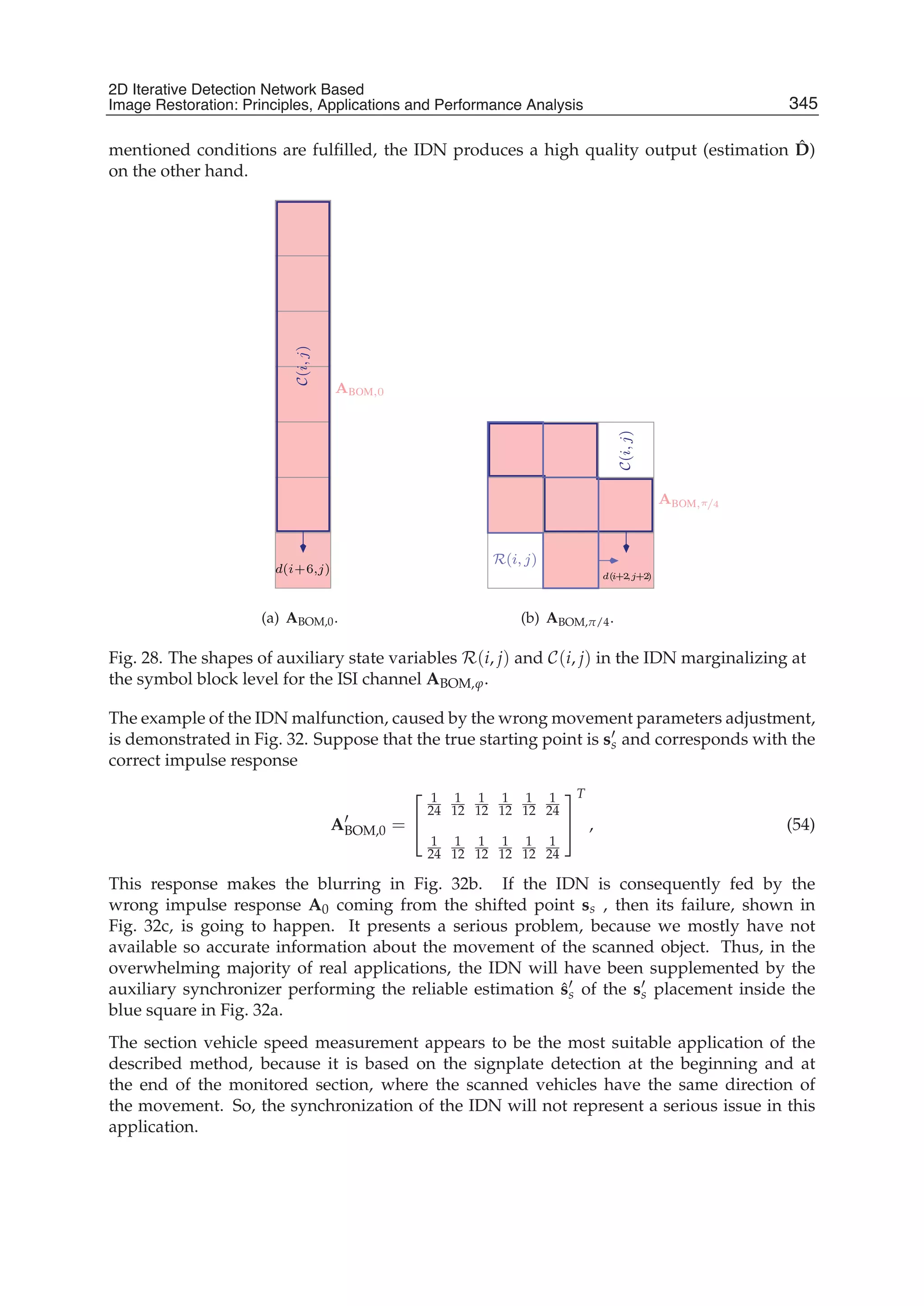
![32 Will-be-set-by-IN-TECH
i − 3
i − 2
i − 1
i
i + 1
i + 2
i + 3
j
(a) The topology of the EN and
IDN.
c(i,j,4)
c(i,j,5)
c(i,j,6)
c(i,j,3)
c(i,j,2)
c(i,j,1)
c(i−3,j,6)
c(i−1,j,5)
c(i−2,j,4)
c(i+2,j,1)
c(i+1,j,2)
c(i+3,j,3)
q(i, j)
d(i, j)
c(i, j, 7)
f( )
B
(b) The EN cell in the node
(i, j).
SI[ˇc(i+2,j,1)]
SO[ˇc(i+2,j,1)]
SO[ˇc(i+1,j,2)]
SI[ˇc(i+1,j,2)]
SO[ˇc(i+3,j,3)]
SI[ˇc(i+3,j,3)]
SI[ˇc(i,j,4)]
SO[ˇc(i,j,4)]
SI[ˇc(i,j,5)]
SO[ˇc(i,j,5)]
SO[ˇc(i,j,6)]
SI[ˇc(i,j,6)]
SI[ˇq(i, j)]
SO[ˇq(i, j)]
SI[ˇc(i, j, 7)]
SO[ˇc(i, j, 7)]
SI[ ˇd(i, j)]
SO[ ˇd(i, j)]
SI[ˇc(i,j,3)]
SO[ˇc(i,j,3)]
SI[ˇc(i,j,2)]
SO[ˇc(i,j,2)]
SI[ˇc(i,j,1)]
SO[ˇc(i,j,1)]
SI[ˇc(i−1,j,5)]
SO[ˇc(i−2,j,4)]
SI[ˇc(i−2,j,4)]
SO[ˇc(i−1,j,5)]
SI[ˇc(i−3,j,6)]
SO[ˇc(i−3,j,6)]
SO[ˇc(i, j, 7)]
SI[ˇc(i, j, 7)]
B−1
f−1( )
(c) The IDN cell in the node (i, j).
Fig. 29. The EN and IDN marginalizing at the symbol level with the centered topology for
the ISI channel ABOM,0.
346 Image Restoration – Recent Advances and Applications](https://image.slidesharecdn.com/imagerestorationrecentadvancesandapplications-160714160024/75/Image-restoration-recent_advances_and_applications-356-2048.jpg)
![2D Iterative Detection Network Based Image Restoration: Principles, Applications and Performace Analysis 33
j − 1 j j + 1
i + 1
i
i − 1
(a) The topology of the EN and IDN.
c(i,j,3)
c(i, j, 4)
c(i,j,5)
c(i,j,6)
c(i+1,j,2)c(i−1,j,5)
c(i, j + 1, 4)
c(i + 1, j + 1, 3)
c(i − 1, j − 1, 6)
c(i, j, 1)
q(i, j)
d(i, j)
c(i, j − 1, 1)
c(i, j, 7)
c(i,j,2)
B
f( )
(b) The EN cell in the node (i, j).
SO[ˇc(i, j, 7)]
SI[ˇc(i, j, 7)]
SO[ˇc(i − 1, j − 1, 6)]
SI[ˇc(i − 1, j − 1, 6)]
SO[ ˇd(i, j)]
SI[ ˇd(i, j)]
SI[ˇc(i, j, 4)]
SO[ˇc(i, j, 4)]
SO[ˇc(i, j − 1, 1)]
SI[ˇc(i, j − 1, 1)]
SO[ˇc(i, j, 7)]
SI[ˇc(i, j, 7)]
SO[ˇc(i,j,5)]
SI[ˇc(i,j,5)]
SO[ˇc(i+1,j,2)]
SI[ˇc(i+1,j,2)]
SI[ˇc(i,j,6)]
SO[ˇc(i,j,6)]
SI[ˇc(i + 1, j + 1, 3)]
SO[ˇc(i + 1, j + 1, 3)]
SO[ˇq(i, j)]
SI[ˇq(i, j)]
SO[ˇc(i, j + 1, 4)]
SI[ˇc(i, j + 1, 4)]
SI[ˇc(i−1,j,5)]
SO[ˇc(i−1,j,5)]
SO[ˇc(i,j,2)]
SI[ˇc(i,j,2)]
SI[ˇc(i,j,3)]
SO[ˇc(i,j,3)]
SI[ˇc(i, j, 1)]
SO[ˇc(i, j, 1)]
B−1
f−1( )
(c) The IDN cell in the node (i, j).
Fig. 30. The EN and IDN marginalizing at the symbol level with the centered topology for
the ISI channel ABOM,π/4.
347
2D Iterative Detection Network Based
Image Restoration: Principles, Applications and Performance Analysis](https://image.slidesharecdn.com/imagerestorationrecentadvancesandapplications-160714160024/75/Image-restoration-recent_advances_and_applications-357-2048.jpg)
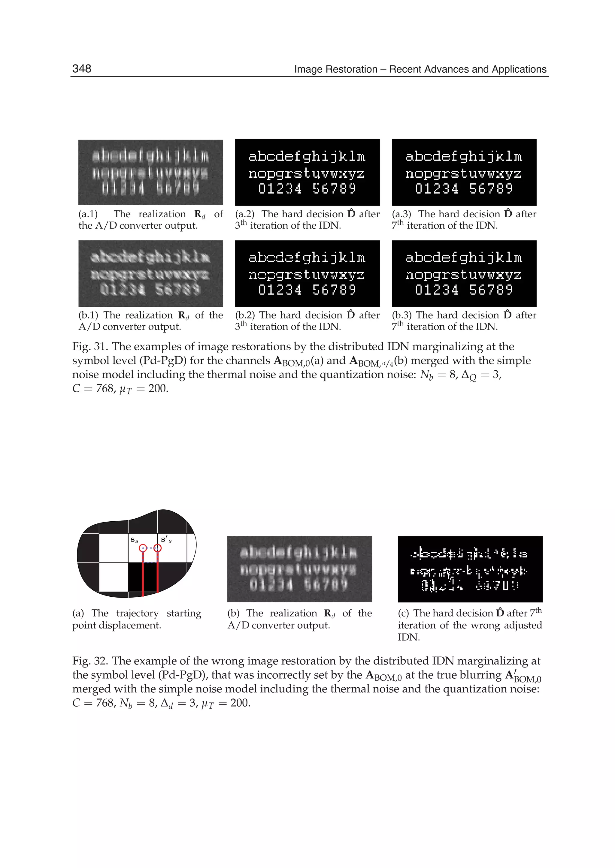
![36 Will-be-set-by-IN-TECH
Vucetic, B. & Juan, J. (2003). Space-Time coding, Kluwer Academic Publishers, ISBN
0-470-84757-3.
Vucetic, B. & Juan, J. (2000). Turbo codes : Principles and Applications, Kluwer Academic
Publishers, ISBN 0-792-37868-7.
Kekrt, D. & Klíma, M. (2008). A black & white picture reconstruction by iterative detection
network in the image capturing system with CCD (CMOS) sensor, 50th International
Symposium ELMAR-2008, Vol. 1, pp. 125-128, ISBN 978-953-7044-06-0, Zadar, Croatia,
September 2008.
Kekrt, D. & Klíma, M. (2008). The iterative detection network based recovery of black &
white pictures shot by camera — implementation and complexity reduction issue,
In Proceedings of the 18th International Conference Radioelektronika 2008, pp. 219-222,
ISBN 978-1-4244-2087-2, Prague, Czech Republic, April 2008.
Kekrt, D. & Klíma, M. (2008). Layered Iterative detection network based text recognition in
the snapshot gained by camera with CCD (CMOS) sensor, In Proceedings of the 12th
International Student Conference on Electrical Engineering POSTER 2008 [CD-ROM],
Prague, Czech Republic, May 2008.
Kekrt, D.; Klíma, M. & Podgorny, R. (2008). The iterative detection network suppression of
defocusing and thermal noise in black and white pictures shot by a camera with
CCD/CMOS sensor, 6th International Conference on Photonics, Devices and Systems,
Vol. 7138, pp. 71381Z-1-71381Z-7, ISBN 978-0-8194-7379-0, Prague, Czech Republic,
August 2008.
Kekrt, D.; Klíma, M. & Fliegel, K. (2008). The iterative detection network based suppression
of the thermal noise and blurring due to object moving in black and white pictures
shot by a camera with CCD/CMOS sensor, In Proceedings of SPIE Optics + Photonics,
Vol. 7076, pp. 70760M-1-70760M-9, ISBN 978-0-8194-7296-0, San Diego, USA, August
2008.
Kekrt, D.; Klíma, M. & Podgorny, R. (2008). Aspects of Image Quality Enhancement in Security
Technology, IEEE International Carnahan Conference on Security Technology 2008, pp.
142-149, ISBN 978-1-4244-1816-9, Prague - Czech Republic, October 2008.
Kekrt, D. & Klíma, M. (2008). The advanced noise model for an IDN based restoration of black
and white pictures captured by a camera with CCD/CMOS sensor, IEEE International
Carnahan Conference on Security Technology 2008, pp. 126-130, ISBN 978-1-4244-1816-9,
Prague, Czech Republic, October 2008.
J. van Vliet L.; Boddeke F. R.; Sudar D. & Young I.T. (1998). Image detectors for digital
image microscopy. M.H.F. Wilkinson, F. Schut (eds.), Digital Image Analysis of Microbes;
Imaging, Morphometry, Fluorometry and Motility Techniques and Applications, Modern
Microbiological Methods, pp. 37-64, John Wiley & Sons, Chichester, The United
Kingdom, 1998.
Anastasopoulos, A. & Chugg, K. (2000). Adaptive soft-input soft-output algorithms for
iterative detection with parametric uncertainty. IEEE Trans. Commun., Vol. 48, pp.
1638-1649, Oct. 2000.
Noels, N.; Herzet, C.; Dejonghe, A.; Lottici, V. ; Steendam, H.; Moeneclaey, M.; Luise, M.;
Vandendorpe, L. (2003). Turbo synchronization : an EM algorithm interpretation,
IEEE International Conference on Communications - ICC, 2003.
350 Image Restoration – Recent Advances and Applications](https://image.slidesharecdn.com/imagerestorationrecentadvancesandapplications-160714160024/75/Image-restoration-recent_advances_and_applications-360-2048.jpg)


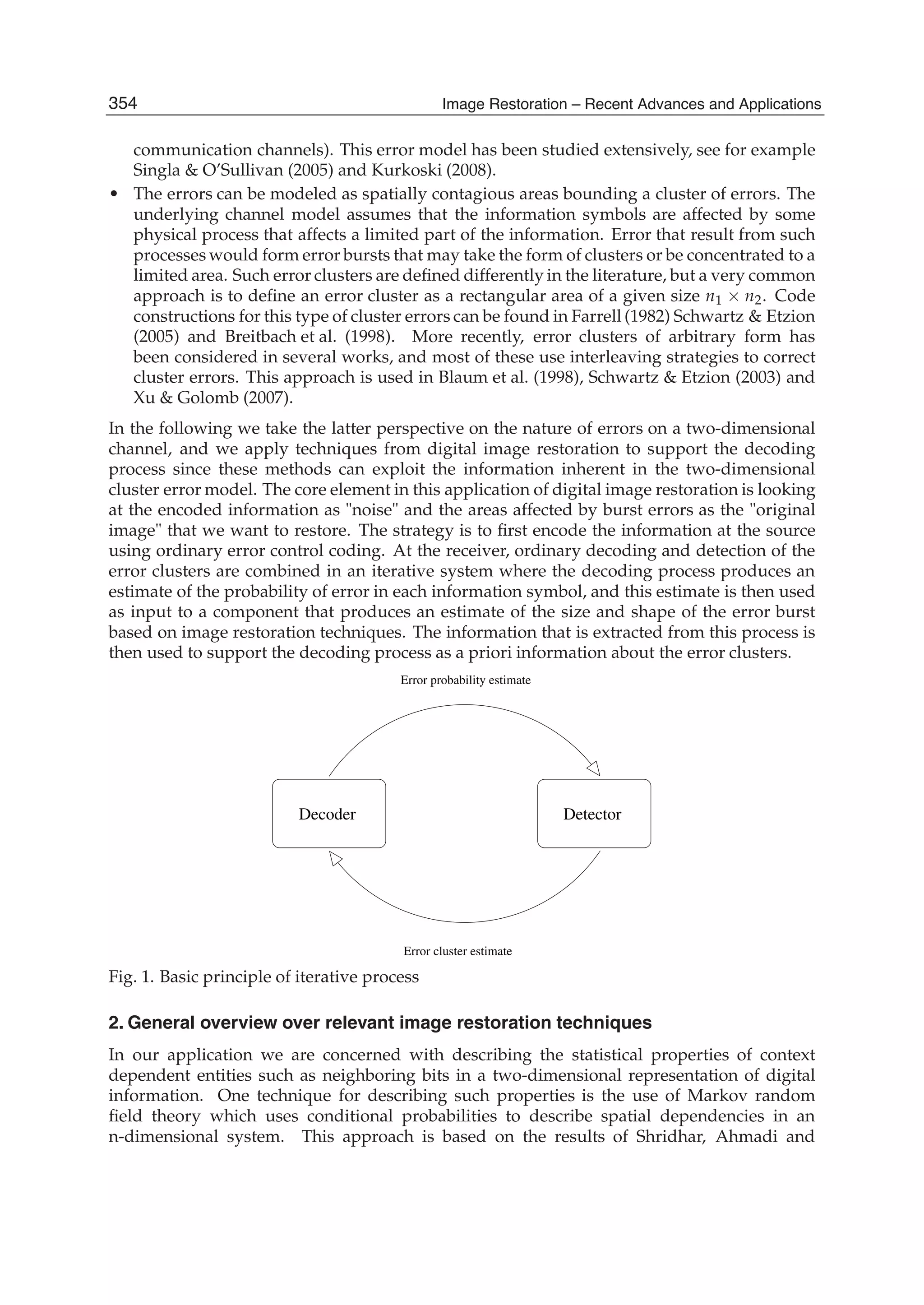

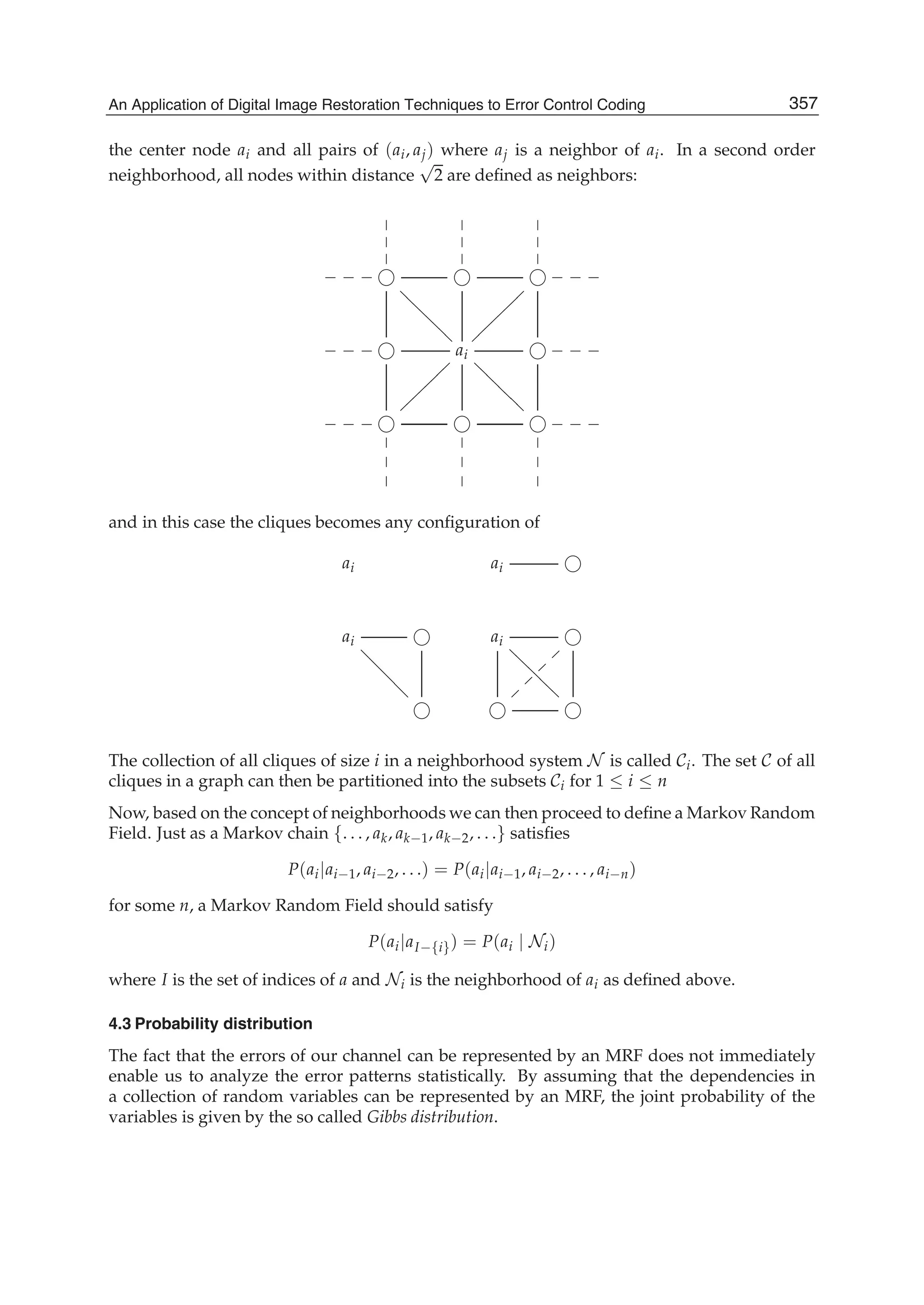
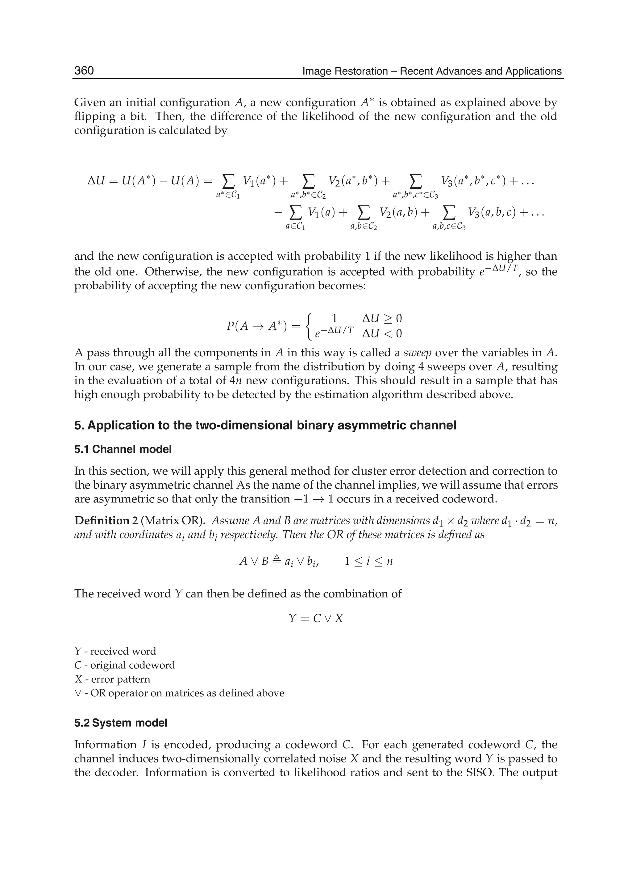
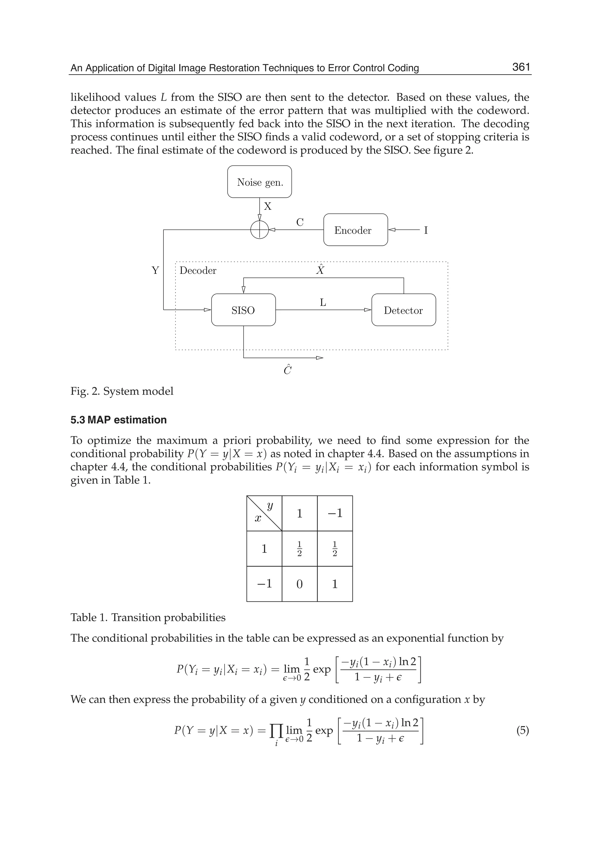
![10 Image Restoration
Substituting (1) and (5) into (4), we can find the joint probability by
P(X = x, Y = y) = Z−1
e− 1
T U(x)
∏
i
lim
→0
1
2
exp
−yi(1 − xi) ln 2
1 − yi +
(6)
Since the natural logarithm is strictly increasing, the following equality holds:
arg max
X
(P(X, Y)) = arg max
X
(ln(P(X, Y))) (7)
In order to avoid computing Z in (6), we take the logarithm of both sides and eliminate
constants to get
V(x) = U(x) + ∑
i
lim
→0
−yi(1 − xi) ln 2
1 − yi +
where V(x) = ln [P(X = x, Y = y)].
We define the partial functions Vi of U(x) according to Li (2000); Shridhar et al. (1989)
V1(xi) = αxi
V2(xi, xi ) = βi,i xixi
V3(xi, xi , xi ) = · · · = 0
Note that the expression for V2 implies that V2(xi, xi ) = βi,i for xi = xi and V2(xi, xi ) =
−βi,i for xi = xi .
From this we get a new expression for V(x):
V(x) = ∑
i
αxi + βi,i ∑
i ∈Ni
xixi + lim
→0
−yi(1 − xi) ln 2
1 − yi +
,
and splitting the last term into a constant and a non-constant term yields
V(x) = ∑
i
αxi + βi,i ∑
i ∈Ni
xixi + lim
→0
xiyi ln 2
1 − yi +
+ lim
→0
−yi ln 2
1 − yi +
.
Since the last term only depends on y, we can find the MAP configuration by simplifying the
expression to:
V(x) = ∑
i
αxi + β ∑
i ∈Ni
xixi + lim
→0
xiyi ln 2
1 − yi +
= ∑
i
α + β ∑
i ∈Ni
xi + lim
→0
yi ln 2
1 − yi +
xi (8)
Having obtained an estimate
ˆX = { ˆX1, . . . , ˆXi, . . . , ˆXn}
362 Image Restoration – Recent Advances and Applications](https://image.slidesharecdn.com/imagerestorationrecentadvancesandapplications-160714160024/75/Image-restoration-recent_advances_and_applications-372-2048.jpg)
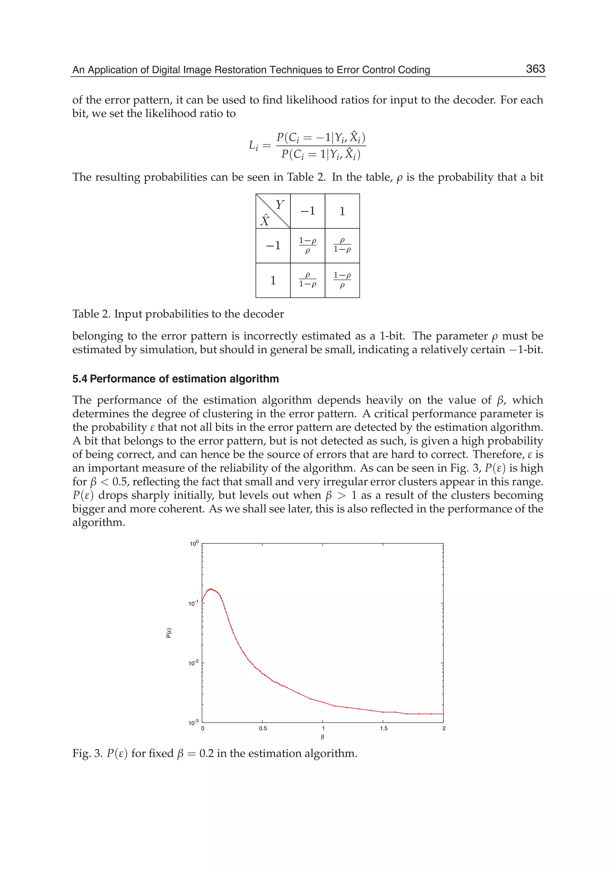
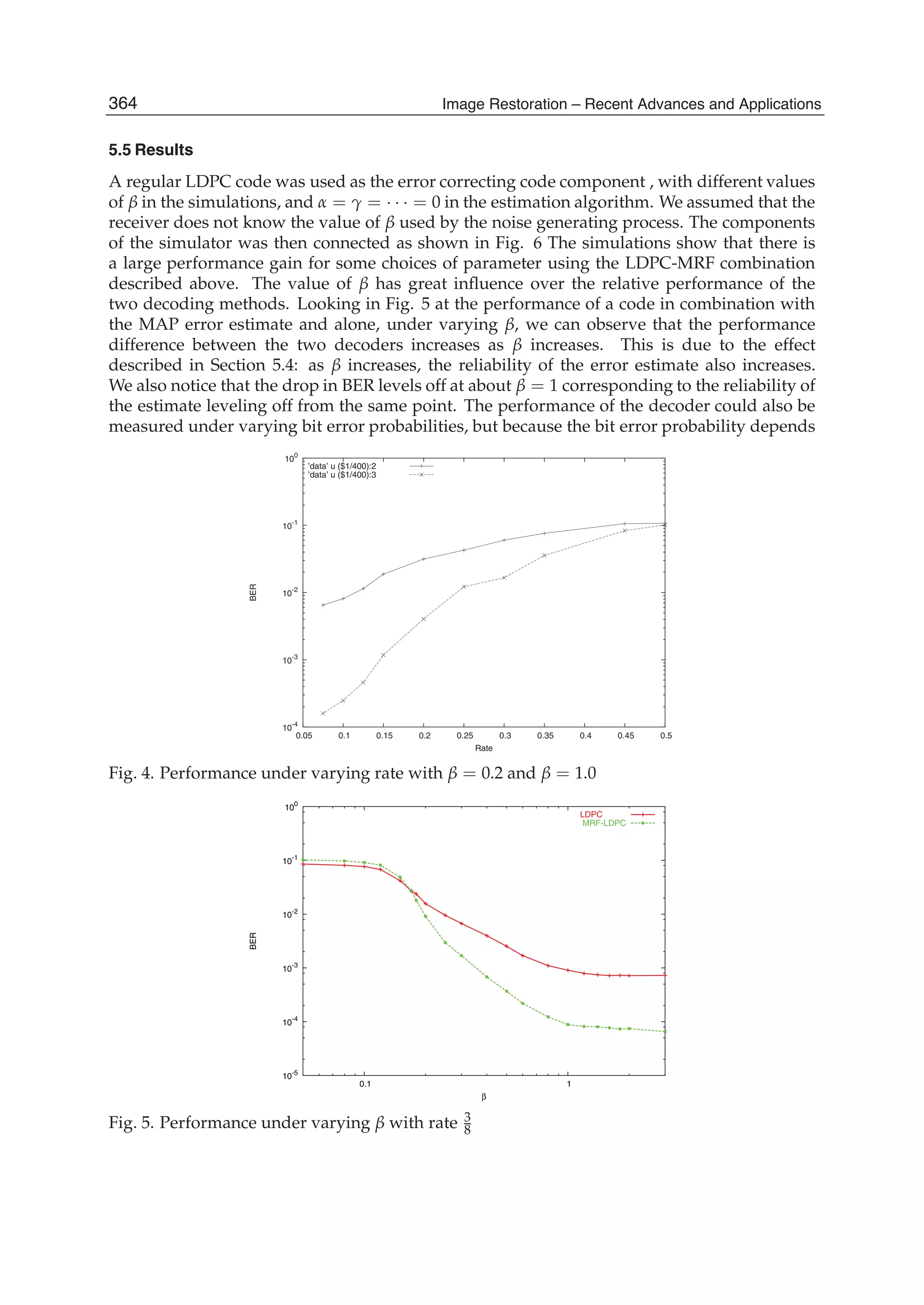

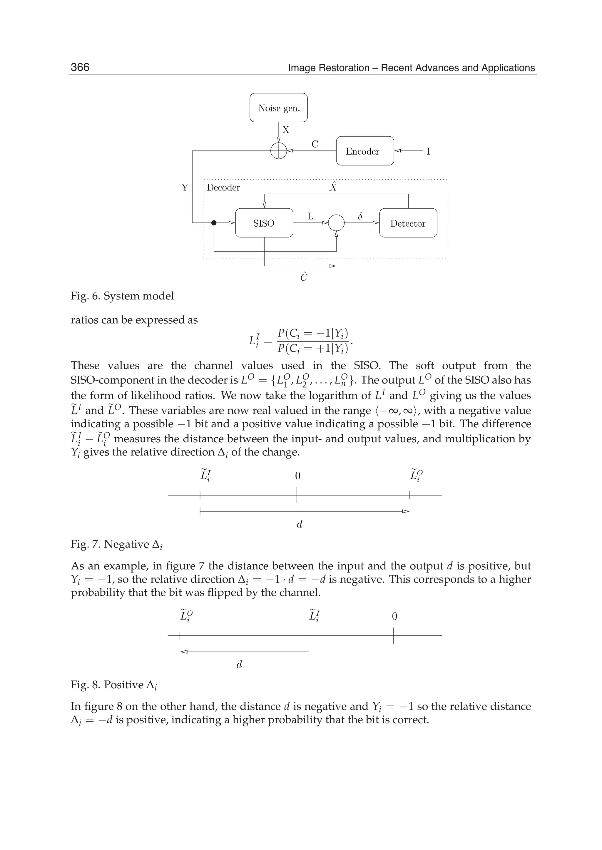
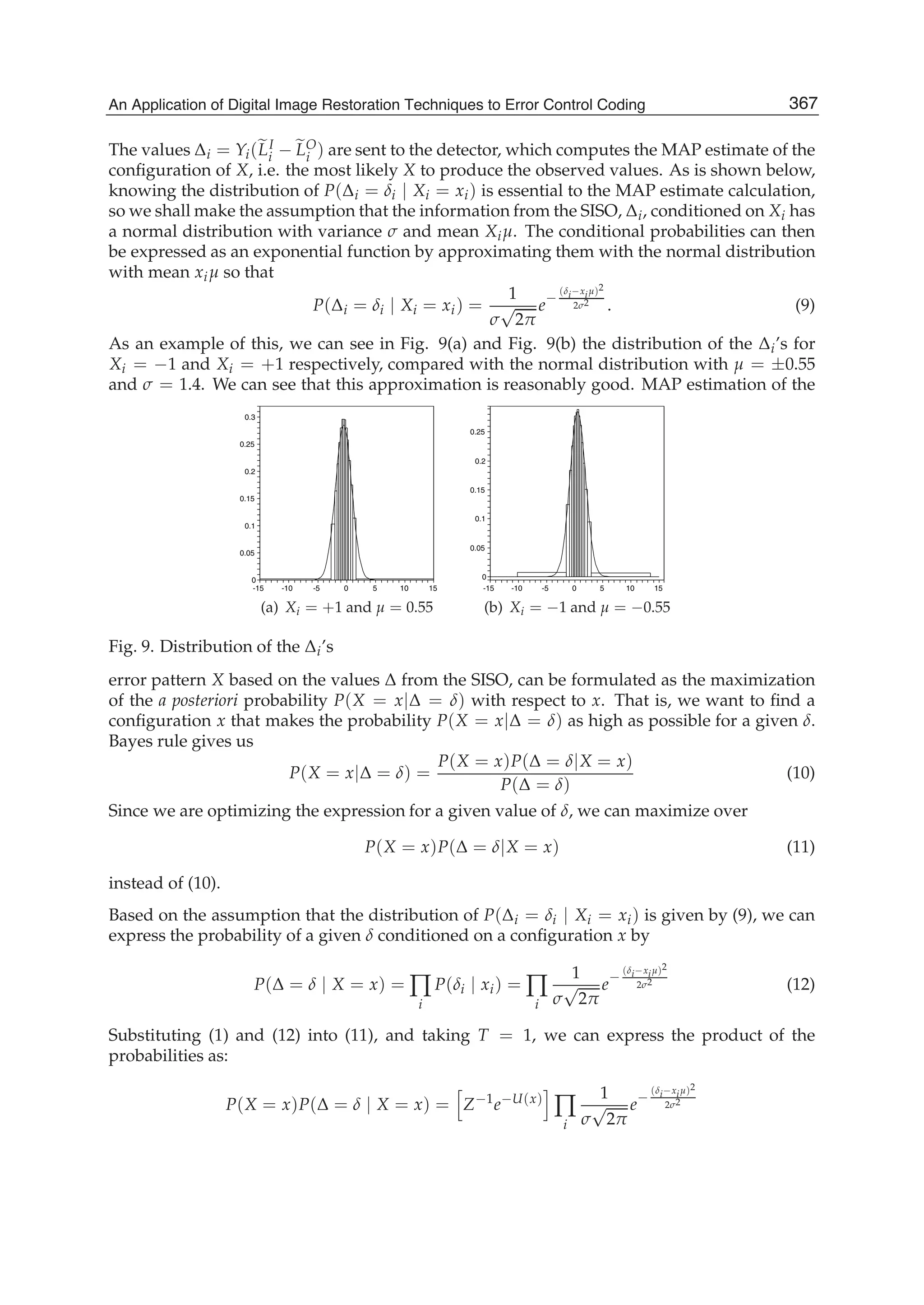
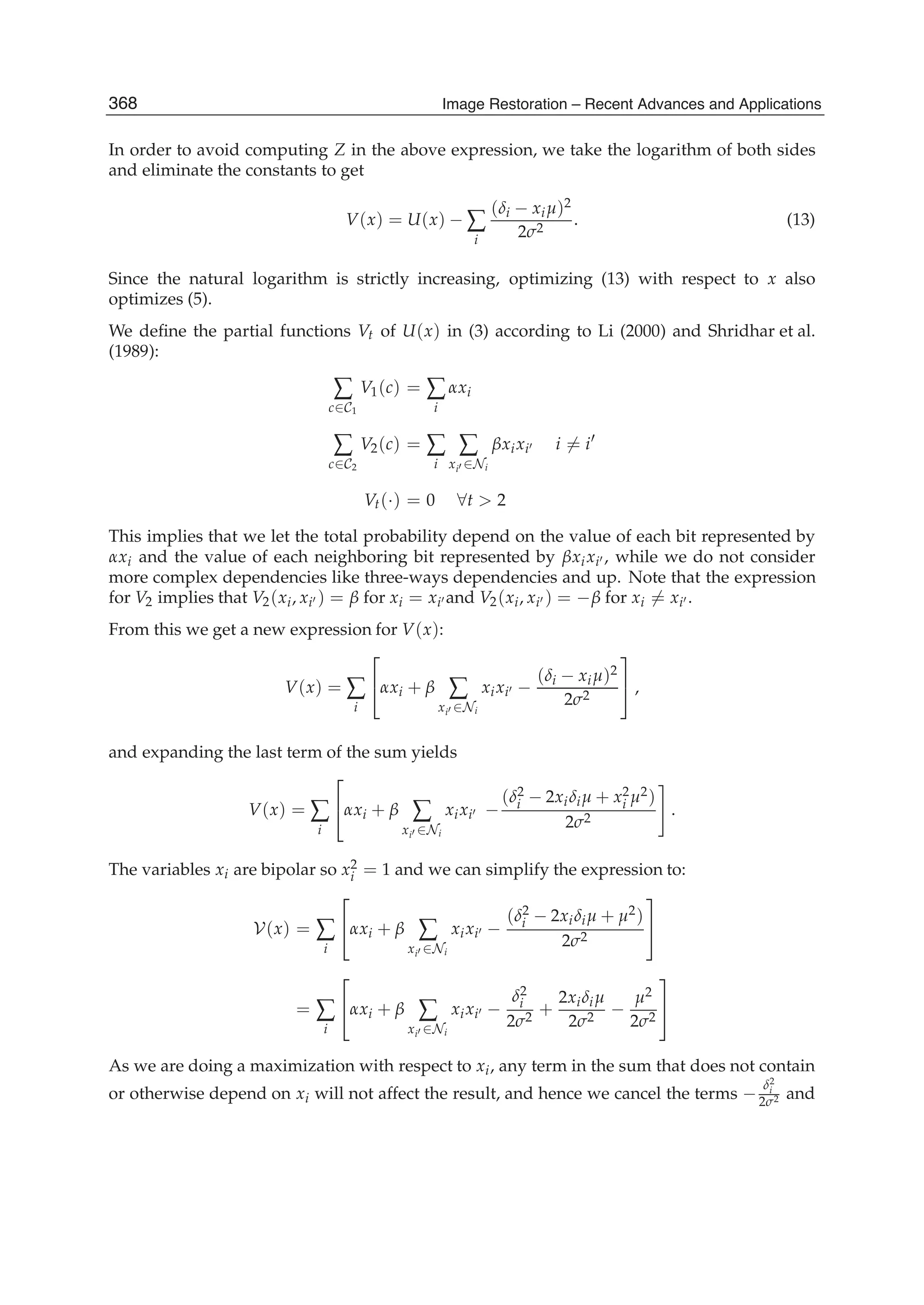
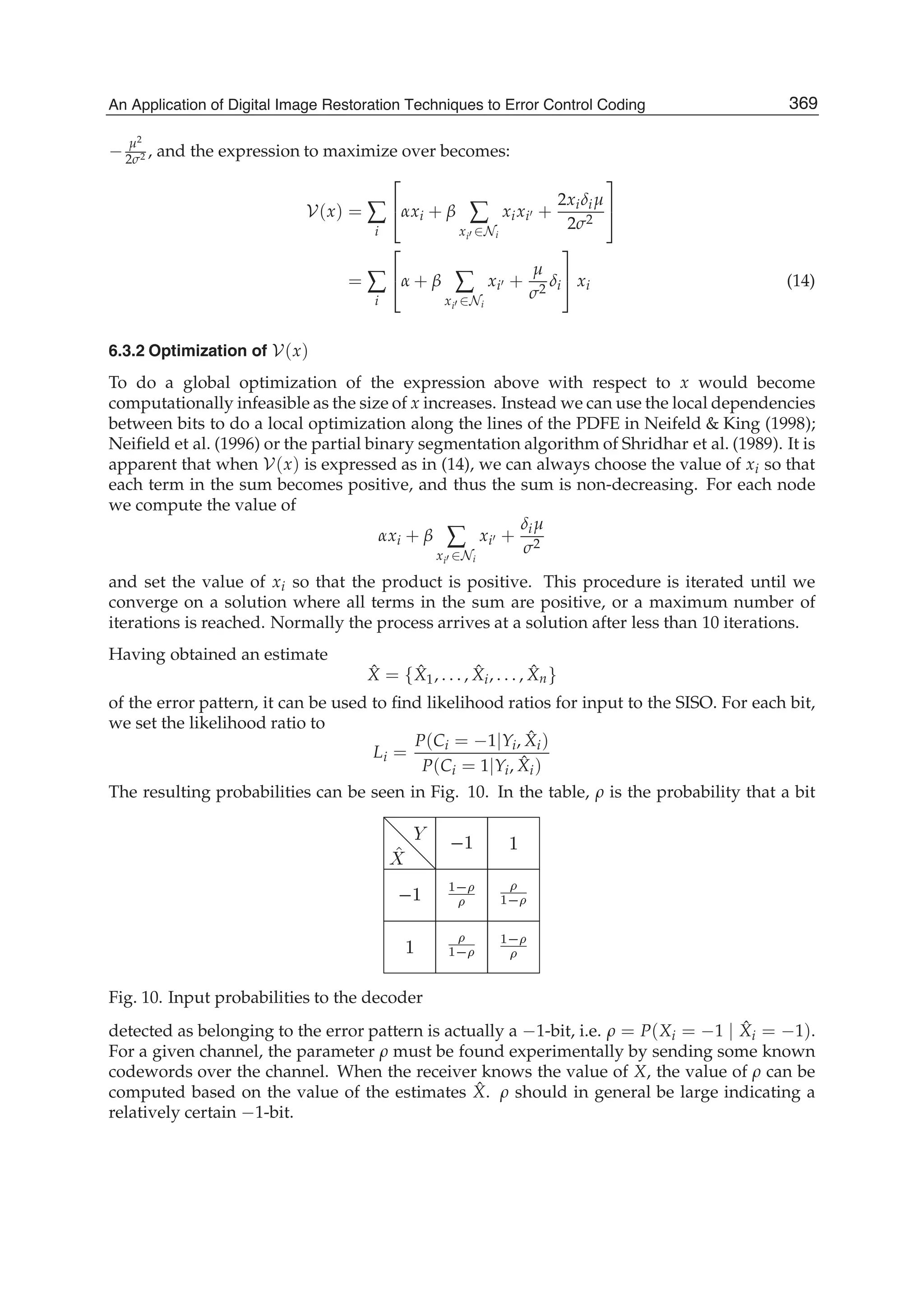
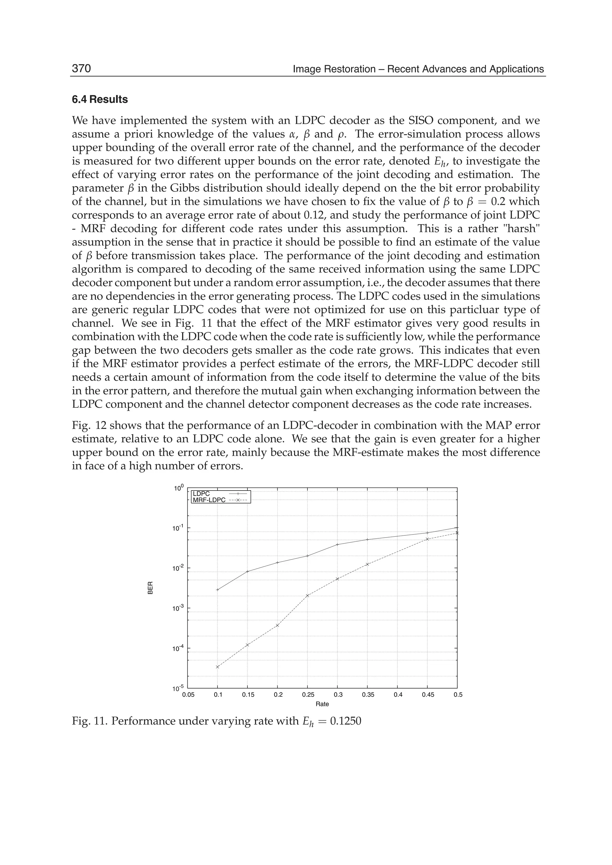
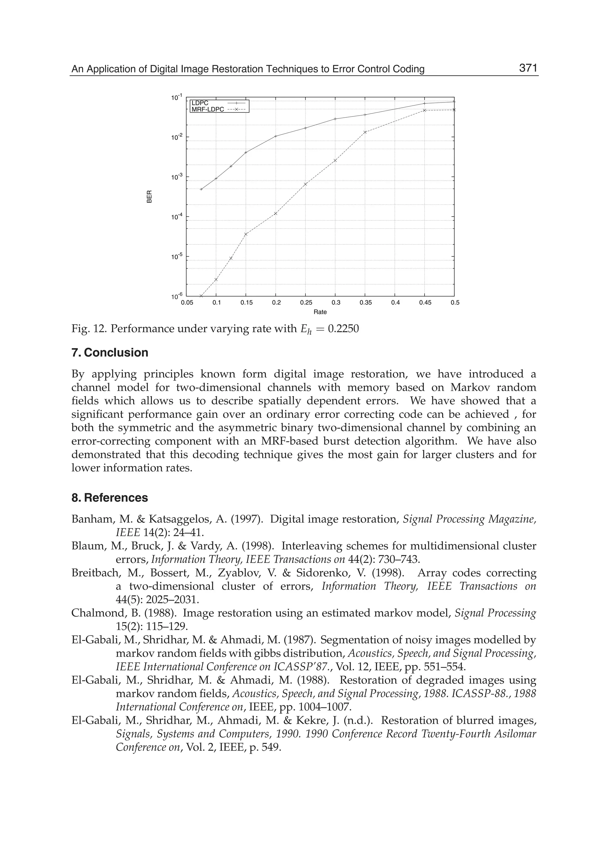

This document discusses image restoration techniques for images degraded by space-variant blurs. It describes running sinusoidal transforms as a method for space-variant image restoration. Running transforms involve applying a short-time orthogonal transform within a moving window, allowing approximately stationary processing. This addresses limitations of methods that assume space-invariance or require coordinate transformations. The chapter presents running discrete sinusoidal transforms as a way to perform the space-variant restoration by modifying orthogonal transform coefficients within the window to estimate pixel values.