Download to read offline
![Line detection - Hough transform (HT)
A line y = mx + n can be represented by a parameter
pair (m, n) which is one point in the parameter space.
You can rewrite the line equation as n = -mx + y. For
a point p = [x, y]T, m and n can vary and form a line in
the parameter space, representing all possible lines
passing through p.](https://image.slidesharecdn.com/test2686-120401060248-phpapp01/85/Test-2-320.jpg)


![[0, 0] j
θ 360°
ρ
.
θ .
.
i 10°
0°
0 10 ... M2 + N2
ρ
discrete image I[i, j] parameter space
In implementation, we usually adopt the polar
representation ρ = j cosθ - i sinθ.](https://image.slidesharecdn.com/test2686-120401060248-phpapp01/85/Test-5-320.jpg)
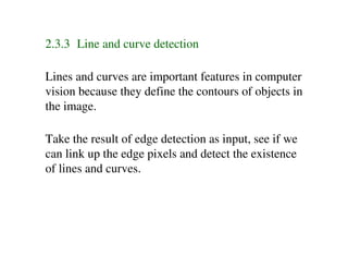
![Line detection algorithm:
• input edge detection result (M x N binary image)
• quantize ρ and θ to create the parameter space,
ρ ∈[0 , M 2 + N 2 ],θ ∈ [ 0 ,2π ]
• initialize all entries of the parameter space to zero
• for each edge point [i, j], increment by 1 each entry
that satisfies the polar representation, e.g. for a
specific quantized value of θ, find the closest
quantized value of ρ
• find the local maxima (ρ, θ), each has the count >
user-defined threshold τ](https://image.slidesharecdn.com/test2686-120401060248-phpapp01/85/Test-6-320.jpg)

![Disadvantages:
• You can generalize HT to detect curve y = f(x, a),
where a = [a1, …, aP]. The parameter space is P-
dimensional. However, search time increases rapidly
with the number of parameters.
• Non-target shapes can produce spurious peaks in
parameter space, e.g. low-curvature curves can be
detected as lines.](https://image.slidesharecdn.com/test2686-120401060248-phpapp01/85/Test-8-320.jpg)
![Another approach to detect line is to fit edge pixels to a
line model - model fitting approach
For a generic line ax + by + c = 0, or , find the
parameter vector [a, b, c]T which results in a line going
as near as possible to each edge point. A solution is
reached when the distance between the line and all the
edge points is minimum – least squares problem.](https://image.slidesharecdn.com/test2686-120401060248-phpapp01/85/Test-9-320.jpg)

![Assume that the set of edge points pi = [xi, yi]T,
i = 1, ...,N belong to a single arc of ellipse
xTa = ax2+bxy+cy2+dx+ey+f = 0
where x = [x2, xy, y2, x, y, 1]T and a = [a, b, c, d, e, f]T.
Find the parameter vector a, associated to the ellipse
which fits p1…pN best in the least squares sense
N 2
min ∑ x i a
T
a
i =1](https://image.slidesharecdn.com/test2686-120401060248-phpapp01/85/Test-11-320.jpg)


![Conversion between RGB and HSI can be implemented
using the MATLAB functions rgb2hsv and hsv2rgb.
An RGB color image in MATLAB corresponds to a
3D matrix of dimensions M x N x 3.
image = imread(filename);
[height, width, color] = size(image);](https://image.slidesharecdn.com/test2686-120401060248-phpapp01/85/Test-20-320.jpg)

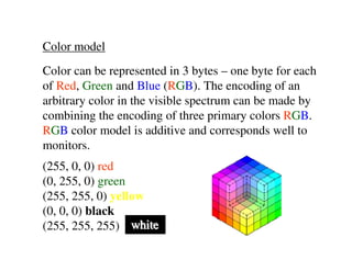
![Histogram can be used to determine how similar a test
image T to a reference image R.
Assume both histograms hT and hR have K bins.
K
intersection = ∑ min(h T [i], h R [i])
i =1
K
∑ min(h T [i], h R [i])
match = i =1
K
∑h
i =1
R [i]
The match value indicates how much color content of
the reference image is present in the test image. It is
relatively invariant to translation, rotation and scale
changes of image.](https://image.slidesharecdn.com/test2686-120401060248-phpapp01/85/Test-23-320.jpg)
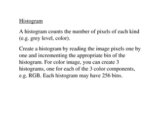
![Sometimes, you may want to compute a dissimilarity
measure
K
distance = ∑ h T [i] − h R [i]
i =1
Noise filtering techniques and edge detectors can be
extended to color images under the componentwise
paradigm.](https://image.slidesharecdn.com/test2686-120401060248-phpapp01/85/Test-24-320.jpg)


![Co-occurrence matrices
A co-occurrence matrix is a 2D array C in which both
the rows and the columns represent a set of image
values (intensities, colors). The value Cd[i, j] indicates
how many times value i co-occurs with value j in some
designated spatial relationship. The spatial relationship
is represented by a vector d = (dr, dc), indicating the
displacement of the pixel having value of j from the
pixel having value of i by dr rows and dc columns.](https://image.slidesharecdn.com/test2686-120401060248-phpapp01/85/Test-30-320.jpg)
![j
1 1 0 0 0 1 2
1 1 0 0 0 4 0 2
0 0 2 2 i 1 2 2 0
0 0 2 2 2 0 0 2
image I C(0,1)
It is common to normalize the co-occurrence matrix
and so each entry can be considered as a probability.
C d [i, j]
N d [i, j] =
∑∑ C d [i, j]
i j](https://image.slidesharecdn.com/test2686-120401060248-phpapp01/85/Test-31-320.jpg)
![Numeric features can be computed from the co-
occurrence matrix that can be used to represent the
texture more compactly.
Energy = ∑∑ N d [i, j]
2
i j
Entropy = −∑∑ N d [i, j]log 2 N d [i, j]
i j
Contrast = ∑∑ (i - j) 2 N d [i, j]
i j
N d [i, j]
Homogeneity = ∑∑
i j 1+ i - j](https://image.slidesharecdn.com/test2686-120401060248-phpapp01/85/Test-32-320.jpg)
![∑∑ (i − µ )(j − µ )N
i j
i j d [i, j]
Correlation =
σiσ j
where µi, µj are the means and σi, σj are the standard
deviations of the row and column sums
N d [i] = ∑ N d [i, j]
j
N d [j] = ∑ N d [i, j]
i](https://image.slidesharecdn.com/test2686-120401060248-phpapp01/85/Test-33-320.jpg)


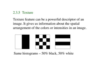
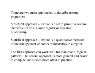
Lines and curves can be detected using techniques like Hough transform and ellipse fitting. Color can be represented in models like RGB or HSI and analyzed using histograms. Texture is described using features such as edgeness, co-occurrence matrices, and statistics like energy, entropy, and contrast computed from the matrices.


![Columbia workshop [ABC model choice]](https://cdn.slidesharecdn.com/ss_thumbnails/columbia-110924060002-phpapp01-thumbnail.jpg?width=640&height=640&fit=bounds)