The study investigates whether improved food legume varieties, particularly faba bean and field pea, enhance technical efficiency in crop production among smallholder farmers in the Bale Highlands of Ethiopia. Despite the importance of legumes in soil regeneration and food security, the findings reveal very low adoption rates of these improved varieties with no significant relationship to efficiency or productivity. The research highlights challenges in mono-cropping systems and raises further questions about agricultural practices in the region.

1. Can improved food legume varieties
increase technical efficiency in crop
production?
A Case Study in Bale Highlands, Ethiopia
Girma T. Kassie, Aden Aw-Hassan, Seid A. Kemal, Luleseged Desta,
Peter Thorne, Kindu Mekonnen, Mulugeta Yitayih
29 September 2016
ILRI, Addis Ababa, Ethiopia

2. Outline
• Motivation
• The key questions
• Methodology
• Results and discussion
• Conclusion and more
questions

3. Motivation
• Faba bean (broad bean), field pea, and lentil are very important
legumes in the highlands of Ethiopia.
• Ethiopia is the largest producer of faba bean in SSA.
• In 2012/13, about 4.4 million smallholder farmers planted 574,000 ha of faba
bean producing 0.9 million tons at an average productivity of 1.6 tons per ha.
• Field pea is also an important source of protein in Ethiopia.
• In 2012, the crop ranked fourth in area coverage with an acreage of 212,890 ha
and annual production of 2.6 million tons (FAO, 2012).
• We all agree (it seems) that legumes are essential for the
regeneration of nutrient‐deficient soils.
• They fix nitrogen!

4. Motivation
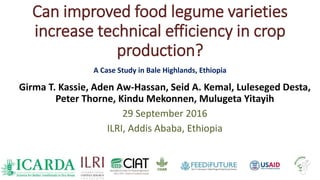
Bale highlands are known for their
mono-cropping production system:
wheat and barley dominated.
Mono-cropping:
• Growing one crop year after year on
the same plot of land
• Non-diverse rotations – Only a
single crop is grown at a time within
a field.
• Associated with two problems:
• Soil degradation
• Increased vulnerability to risk
• Implies lower efficiency [broadly
defined] compared to poly-cropping
systems.

5. The key questions
• Our questions
• How efficient are improved faba bean and field pea growers compared
to non-growers?
• If there is a considerable difference in efficiency, can we attribute this
to the inclusion of improved faba bean and field pea varieties?
• Does crop productivity [crop output per unit of the most limiting
input] vary between improved faba bean and field pea growers and
non-growers?
• Our objective
• To empirically show whether the adoption of improved food legume
varieties increases the technical efficiency of crop production.

6. Methodology
•Sampling
• Multi-stage (mixed) sampling
• 3 of the 4 major legume producing districts in Bale highlands
were selected.
• Agarfa, Goba and Sinana based on relative importance of
food legumes in terms of land allocation for crops.
• 4 peasant associations in each district were selected
randomly.
• 200 farm households were randomly selected from the 4
PAs/District.
• Total sample size 600 farm HHs.

7. Analytical framework
1. Efficiency analysis (SF Model)
N,..,2i,xy iii  
iii uv 
),0(Ν~v 2
vi 
F~ui
yi is log of total crop yield
xi vector of (log of) inputs
εi composite error
υi idiosyncratic error (iid)
ui inefficiency (one-side disturbance)
The assumption about the distribution (F) of ui term is needed to make the model
estimable. Four options so far:
1. Half normal distribution ui ~ N+(0, σu
2) (Aigner et al., 1977).
2. Exponential distribution ui ~ ε(σu) (Meesun and van den Broeck ,1977)
3. Truncated normal (Stevenson, 1980)
4. Gamma distribution (Greene, 1980, 2003).

8. SF Model (2)
• Two step estimation
1- estimates of the model parameters ĥ are obtained by
maximizing the LL-function l(ĥ)
2 – point estimates of inefficiency can be obtained thru the
mean (or the mode) of the conditional distribution
where
• Post-estimation procedures to compute efficiency
parameters:
– Jondrow et al (1982): TEi = 1-E[ui|εi]
– Battese and Coelli (1988): TEi = E[exp(-ui|εi)]
)ˆ|u(f ii 
 ˆxˆyˆ iii 

9. SFA models
–Y= bread wheat equivalent in birr
– Efficiency model 1
• Stoc. frontier normal/tnormal model
• Jondrow et al (1982)
– Efficiency model 2
• Stoc. frontier normal/tnormal model
• Battese and Coelli (1988)
– Efficiency model 3
• Stoc. frontier normal/exponential model
• Jondrow et al (1982)
– Efficiency model 4
• Stoc. frontier normal/exponential model
• Battese and Coelli (1988)

10. Analytical framework
2. Impact analysis
Where δi is impact [technical efficiency] on individual ‘i’;
A
iY Is potential outcome of adoption for individual ‘i’.
Is potential outcome of non-adoption for individual ‘i’.
N
iY
Let D denotes adoption decision (assumed to be binary) and
takes the value 1 for adopters (A) and 0 for non adopters (N).
N
i
A
ii YY 

11. 2. Impact analysis







0DifY
1DifY
Y
i
N
i
i
A
i
i
)(*)(*][][ 01  DPATUDPATETYYEEATE N
i
A
ii
]1|[]1|[]1|[  i
N
ii
A
iii DYEDYEDEATET 
]0D|Y[E]0D|Y[E]0D|[EATU i
N
ii
A
iii  
ATET is identified only if E[YN|D=1]-E[YN|D=0]=0: That is the TEs of HHs
from the adopter and non-adopter groups would not differ in the
absence of the improved food legume varieties.
][ iD YEPOM 

12. 2. Impact analysis
• In population terms, the average trt effect (ATE) is
• ATE = E[TEadopt – TEnonadopt] = E[TEadopt] – [TEnonadopt]
• Missing data problem – we only observe one of the potential outcomes:
– We observe TEadopt for adopting farm HHs.
– We observe TEnonadopt for non-adopting farm HHs.
• When the adoption level/treatment [0/1] is randomly assigned to farm HHs,
the potential outcomes are independent of the adoption level [0/1] .
– Assuming that adoption level [0/1] is randomly assigned is hardly convincing.
• Rather, we assume that adoption level is as good as randomly assigned after
conditioning on covariates. This is called conditional independence.
• In fact, we need only conditional mean independence [CMI] – that is after
conditioning on covariates, the adoption level does not affect the means of the
potential outcomes.
– CMI restricts the dependence b/n adoption model and the potential outcomes

13. 2. Impact analysis
• Overlap assumption
– This ensures that each individual could get any adoption level.
• IID assumption
– This ensures that the potential outcomes and adoption level of each
farm HH are unrelated to potential outcomes and adoption levels of
all the other farm HHs in the population.
• Practically speaking, assuming independence of observations suffices.

14. 2. Impact analysis
• Given the fact that the potential outcomes framework formulates
the estimation of the ATE as a missing data problem, the
parameters of an auxiliary model can be used to solve it.
– The auxiliary model is how we condition on covariates so that the trt is as
good as randomly assigned:
Model Estimator
Outcome → Regression adjustment (RA)
Treatment → Inverse-probability weighted (IPW)
Outcome and treatment → Augmented IPW (AIPW)
Outcome and treatment → IPW RA
Treatment → Propensity score matching
Outcome (non-parametrically) → Nearest-neighbor matching

15. Treatment-effects estimators employed
• Adjustment and weighting
– Regression adjustment [see: Lane and Nelder (1982); Cameron and Trivedi (2005, chap. 25);
Wooldridge (2010, chap. 21); and Vittinghoff, Glidden, Shiboski, and McCulloch (2012, chap. 9).]
– Inverse probability weighting [see: Imbens (2000); Hirano, Imbens, and Ridder (2003); Tan
(2010); Wooldridge (2010, chap. 19); van der Laan and Robins (2003); and Tsiatis (2006, chap. 6).]
– Inverse probability weighting with regression adjustment (IPWRA) [see:
Wooldridge, 2007; Wooldridge, 2010]
– Augmented inverse probability weighting (AIPW) [see:Robins, Rotnitzky, and
Zhao (1995); Bang and Robins (2005); Tsiatis (2006) and Tan (2010).]
• Matching estimators
– Nearest neighbor matching [see: Abadie et al. (2004); Abadie and Imbens (2006,
2011)].
– Propensity score (treatment probability) matching [See: Rosenbaum and
Rubin (1983); Abadie and Imbens (2012)].

16. Results and
Discussion

17. Description of the sample population
• HHs – 90% male headed and 10% female headed.
• Average land holding/hhd: 2.81 ha (reported)
• On average 37% of the farm plot is allocated to faba bean and 12% for field
pea by the sample households.
• Legume producers
• Faba bean: 50.95%
• Field pea: 31.37%
• Faba bean or field pea: 67.76%
• Adopters of improved faba bean and field pea varieties:
• Improved faba bean or field pea: 23.13%

18. SFA model results
Variable Model 1 Model 2 Model 3 Model 4
Frontier
lncultland 0.182*** (3.36) 0.17*** (2.93) 0.182*** (3.36) 0.17*** (2.93)
lnhumlabor -0.029 (-1.65) -0.013 (-.75) -0.029 (-1.65) -0.013 (-0.75)
Lnoxenlabor 0.308*** (7.41) 0.285*** (6.63) 0.308*** (7.41) 0.285*** (6.63)
Lntotureadapbiofe 0.027** (2.58) 0.034*** (3.25) 0.027** (2.58) 0.034*** (3.25)
Lnherbic 0.28*** (5.39) 0.27*** (5.28) 0.28*** (5.39) 0.27*** (5.29)
Lnfungic 0.18*** (4.9) 0.169*** (4.64) 0.18*** (4.9) 0.169*** (4.64)
Lnmachintime 0.067*** (7.05) 0.063*** (6.71) 0.067*** (7.05) 0.063*** (6.71)
Constant -0.291**(-2.47) -0.239* (-1.86) -0.291** (-2.48) -0.24* (-1.87)
_μ -404.25 (-53.75) -362.15 (-20.57)
σu 4.76 (34.66) 4.54 (24.49) -2.49(-9.62) -2.71 (-8.81)
σv -2.19 (-15.51) -2.08 (-15.4) -2.192 (-15.46) -2.07 (-15.38)
Statistics
N 575 575 575 575
LL -332.62 -335.08 -332.61 -335.07
AIC 687.24 692.16 685.22 690.14
BIC 735.14 740.06 728.76 733.68

19. The outcome variables
Variable N Mean Std. Dev. Min Max
Efficiency measure 1 575 0.781 0.108 0.094 0.937
Efficiency measure 2 575 0.794 0.103 0.101 0.939
Efficiency measure 3 575 0.782 0.108 0.094 0.937
Efficiency measure 4 575 0.794 0.103 0.100 0.939
Total bread wheat eqvt (kcl/ha) 575 2.936 2.993 0.030 29.872
Total bread wheat eqvt (birr/ha) 575 3.047 3.137 0.030 31.648

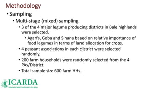
20. Simple comparison of adopters and non-adopters02468
0 .2 .4 .6 .8 1
Technical efficiency via E[exp(-u)|e] (BC approach)
Non-adopter
Adopter
kernel = epanechnikov, bandwidth = 0.0221
Kernel density estimate
0246
Density
0 .2 .4 .6 .8 1
Technical efficiency via exp[-E(u|e)] (JLMS - approach)
Non-adopter
Adopter
kernel = epanechnikov, bandwidth = 0.0241
Kernel density estimate

21. Simple comparison of adopters and non-adopters0
.1.2.3
0 10 20 30
Total bread wheat equivalent (kcal) per hectare
Non-adopter
Adopter
kernel = epanechnikov, bandwidth = 0.4076
Kernel density estimate
0
.1.2.3
Density
0 10 20 30
Total bread wheat equivalent (birr) per hectare
Non-adopter
Adopter
kernel = epanechnikov, bandwidth = 0.4010
Kernel density estimate

22. Average trt effect and Average trt effect on the treated
RA
β(Z)
IPW
β(Z)
AIPW
β(Z)
IPWRA
β(Z)
NNMATCH
β(Z)
PSMATCH
β(Z)
Efficiency measure 1
ATET
-.004 (-0.27) -.003 (-0.25) -0.006 (-.48) -.008 (-.51) -.010 (-.69)
ATE
.002 (0.16) -.01 (-0.49) 0.002 (0.07) 0.006 (0.56) 0.016 (1.01) -.001 (-.04)
Efficiency measure 2
ATET
-.004 (-0.35) -.003 (-0.3) -0.006 (-.52) -.008 (-.54) -0.009(-.69)
ATE
.001 (0.07) -.01 (-0.52) 0.002(0.08) 0.005 (0.50) 0.014 (0.95) -.002(-.09)
Efficiency measure 3
ATET
-.004 (-0.28) -.003 (-0.25) -0.006 (-.46) -.008 (-.51) -.010 (-.69)
ATE
.002 (0.16) -.01 (-0.49) 0.002 (0.07) 0.006 (0.55) 0.016 (1.01) -.001 (-.04)
Efficiency measure 4
ATET
-.004 (-0.35) -.003 (-0.3) -0.006 (-.52) -.008 (-.54) -0.009(-.69)
ATE
.001 (0.07) -.01 (-0.52) 0.002(0.08) 0.005 (0.49) 0.014 (0.95) -.002(-.09)
Total bread wheat eqvt (kcl/ha)
ATET .088 (0.33) -.067 (-.16) -.298 (-.99) 0.337 (1.03) -.778 (-1.13)
ATE
-.109 (-.44) -.392 (-1.50) -.194 (-.72) -.298 (-1.51) 0.117 (0.49) -.113 (-.31)
Total bread wheat eqvt (birr/ha) ATET
0.171(0.59) -.046 (-.09) -.180 (-.55) 0.510 (1.59) -1.034 (-1.08)
ATE
-.053(-.20) -.364 (-1.21) -.151 (-.49) -.264 (-1.25) 0.215 (0.92) -.109 (-.26)
This would have meant: For
the farm HHs who are
adopting, TE of crop
production is 0.004 less than
if none of these farm HHs
adopted.
This would have meant :
When all farmers adopt, TE of
crop production is estimated
to be 0.002 units higher than
when no farm HH adopts.

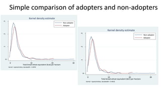
23. Conclusions and further questions
• Very low adoption of improved legume varieties – particularly faba
bean and field pea.
• No relationship with efficiency no matter how the latter was
measured.
• No relationship with productivity per unit of limiting factor no
matter what conversion [energy or price] was used.
•We observed that complementary inputs are not being
used as per the recommendations.

24. Conclusions and further questions
• Human labor is not rewarding in crop production in the
study area. Legumes are still dependent on human labor.
Would they have any future in mechanized farming?
• Would simply disseminating the ‘improved varieties’
help? How?
•Bale highlands is known for farmers heavily dependent
on machinery for their crop production. How will
legumes – produced manually – fit into this system?
• Are they meant to continue as break crops?

25. Thank You so much!!