MY notes on risk

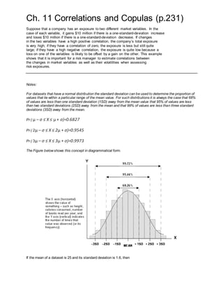
1. Ch. 11 Correlations and Copulas (p.231)
Suppose that a company has an exposure to two different market variables. In the
case of each variable, it gains $10 million if there is a one-standard-deviation increase
and loses $10 million if there is a one-standard-deviation decrease. If changes
in the two variables have a high positive correlation, the company’s total exposure
is very high; if they have a correlation of zero, the exposure is less but still quite
large; if they have a high negative correlation, the exposure is quite low because a
loss on one of the variables is likely to be offset by a gain on the other. This example
shows that it is important for a risk manager to estimate correlations between
the changes in market variables as well as their volatilities when assessing
risk exposures.
Notes:
For datasets that have a normal distribution the standard deviation can be used to determine the proportion of
values that lie within a particular range of the mean value. For such distributions it is always the case that 68%
of values are less than one standard deviation (1SD) away from the mean value that 95% of values are less
than two standard deviations (2SD) away from the mean and that 99% of values are less than three standard
deviations (3SD) away from the mean.
Pr ( μ – σ ≤ X ≤ μ + σ)=0.6827
Pr ( 2μ – σ ≤ X ≤ 2μ + σ)=0.9545
Pr ( 3μ – σ ≤ X ≤ 3μ + σ)=0.9973
The Figure belowshows this concept in diagrammatical form.
If the mean of a dataset is 25 and its standard deviation is 1.6, then

2. 1. 68% of the values in the dataset will lie between MEAN-1SD (25-1.6=23.4)
and MEAN+1SD (25+1.6=26.6)
2. 99% of the values will lie between MEAN-3SD (25-4.8=20.2) and MEAN+3SD (25+4.8=29.8).
If the dataset had the same mean of 25 but a larger standard deviation (for example, 2.3) it would indicate
that the values were more dispersed. The frequency distribution for a dispersed dataset would still show a
normal distribution but when plotted on a graph the shape of the curve will be flatter as in figure 4.
Limitations:
Knowing thelimitationsof a simple linear regression model A simple linear regression model is just what
it says it is: simple. I don’t mean easy to work with, necessarily, but simple in the uncluttered sense. The
model tries to estimate the value of y by only using one variable, x. However, the number of real-world
situationsthatcan be explained by using a simple, one-variablelinearregression is small.Oftentimesone
variablejustcan’tdo all the predicting.If onevariablealone doesn’tresultin a model that fits, add more
variables.Oftentimesit takesmany variablesto make a good estimate for y. In the case of stock market
prices, they’re still looking for that ultimate prediction model. As another example, health insurance
companies try to estimate how long you will live by asking you a series of questions (each of which
representsa variablein the regression model).You can’tfind one singlevariable thatestimateshow long
you’lllive; you mustconsidermany factors:yourhealth,yourweight,whether or not you smoke, genetic
factors, how much exercise you do each week, and the list goes on and on and on. The point is,
regression models don’t always use just one variable, x, to estimate y. Some models use two, three, or
even more variables to estimate y. Those models aren’t called simple linear regression models; they’re
called multiple linear regression models.
This chapter explains how correlations can be monitored in a similar way to volatilities. It also covers what
are known as copulas. These are tools that provide away of defining a correlation structure between two
or more variables, regardless of the shapes of their probability distributions. Copulas have a number of
applications in risk management. The chapter shows how a copula can be used to create a model
of default correlation for a portfolio of loans. This model is used in the Basel II capital requirements.

3. I. CorrelationCoefficient
11.1 DEFINITION OF CORRELATION
The coefficient of correlation, ρ, between two variables V1 and V2 is defined as
ρ =E(V1V2) − E(V1)E(V2)
SD(V1)SD(V2)
(11.1)
where E(.) denotes expected value and SD(.) denotes standard deviation. If there is
no correlation between the variables, E(V1V2) = E(V1)E(V2) and ρ = 0. If V1 = V2,
both the numerator and the denominator in the expression for ρ equal the variance
of V1. As we would expect, ρ = 1 in this case. The covariance between V1 and V2 is defined as
cov(V1,V2) = E(V1V2) − E(V1)E(V2)
The distinction is subtle but important:
1. The average value is a statistical generalization of multiple occurrences of an event (such as the
mean time you waited at the checkout the last 10 times you went shopping, or indeed the mean
time you will wait at the checkout the next 10 times you go shopping).
2. The expected value refers to a single event that will happen in the future (such as the amount of
time you expect to wait at the checkout the next time you go shopping - there is a 50% chance it
will be longer or shorter than this). The expected value is numerically the same as the average
value, but it is a prediction for a specific future occurrence rather than a generalization across
multiple occurrences.
You are thinking about investing your money in the stock market. You have the following two
stocks in mind: stock A and stock B. You know that the economy can either go in recession or it
will boom. Being an optimistic investor, you believe the likelihood of observing an economic
boom is two times as high as observing an economic depression. You also know the following
about your two stocks:
State of the
Economy
Probability RA RB
Boom 10% –2%
Recession 6% 40%

4. a) Calculate the expected return for stock A and stock B
b) Calculate the total risk (variance and standard deviation) for stock A and for stock B
c) Calculate the expected return on a portfolio consisting of equal proportions in both stocks.
d) Calculate the expected return on a portfolio consisting of 10% invested in stock A and the
remainder in stock B.
e) Calculate the covariance between stock A and stock B.
f) Calculate the correlation coefficient between stock A and stock B.
g) Calculate the variance of the portfolio with equal proportions in both stocks using the
covariance from answer e.
h) Calculate the variance of the portfolio with equal proportions in both stocks using the
portfolio returns and expected portfolio returns from answer c.
ANSWER
a) p(boom) = 2/3 and p(recession)=1/3 (Note that probabilities always add up to 1)
E(RA) = 2/3 × 0.10 + 1/3 × 0.06 = 0.0867 (8.67%)
E(RB) = 2/3 × -0.02 + 1/3 × 0.40 = 0.12 (12%)
b) SD(RA) = [2/3 × (0.10-0.0867)2 + 1/3 × (0.06-0.0867)2]0.5= 0.018856 (1.886%)
SD(RB) = [2/3 × (-0.02-0.12)2 + 1/3 × (0.40-0.12)2]0.5 = 0.19799 (19.799%)
c) Portfolio weights: WA=0.5 and WB=0.5:
E(RP) = 0.5 × 0.0867 + 0.5 × 0.12 = 0.10335 (10.335%)
d) Portfolio weights: WA=0.1 and WB=0.9:
E(RP) = 0.1 × 0.0867 + 0.9 × 0.12 = 0.11667 (11.667%)
e) COV (RA,RB) =
2/3 × (0.10-0.0867) × (-0.02-0.12) + 1/3 × (0.06-0.0867) × (0.40-0.12) = –0.0037333
f) CORR(RA,RB) = –0.0037333 / (0.018856 × 0.19799) = –1 (Rounding! Remember the
correlation coefficient cannot be less than –1)

5. g) VAR(RP) = 0.52 × 0.0188562 + 0.52 × 0.197992 + 2 × 0.5 × 0.5 × –0.0037333 =
–0.008022
SD(RP) = 8.957%
h) E(RP|Boom) = 0.5 × 0.10 + 0.5 × -0.02 = 0.04 (4%)
E(RP|Recession) = 0.5 × 0.06 + 0.5 × 0.40 = 0.23 (23%)
Hence, E(RP) = 2/3 × 0.04 + 1/3 × 0.23 = 0.10335 (10.335%)
And, SD(RP) = [2/3 × (0.04-0.10335)2 + 1/3 × (0.23-0.10335)2]0.5 = 0.08957 (8.957%)
Calculating Covariance
Calculating a stock's covariance starts with finding a list of previous prices. This is
labeled as "historical prices" on most quote pages. Typically, the closing price for each
day is used to find the return from one day to the next. Do this for both stocks and build
a list to begin the calculations.
For example:
Day A Returns (%) B Returns (%)
1 1.1 3
2 1.7 4.2
3 2.1 4.9
4 1.4 4.1
5 0.2 2.5
Table 1: Daily returns for two stocks using
the closing prices
From here, we need to calculate the average return for each stock:
For A it would be (1.1 + 1.7 + 2.1 + 1.4 + 0.2) / 5 = 1.30
For B it would be (3 + 4.2 + 4.9 + 4.1 + 2.5) / 5 = 3.74
Now, it is a matter of taking the differences between A's return and A's average return,
and multiplying it by the difference between B's return and B's average return. The last

6. step is to divide the result by the sample size and subtract one. If it was the
entire population, you could just divide by the population size.
This can be represented by the following equation:
Using our example on A and B above, the covariance is calculated as:
= [(1.1 - 1.30) x (3 - 3.74)] + [(1.7 - 1.30) x (4.2 - 3.74)] + [(2.1 - 1.30) x (4.9 - 3.74)] + …
= [0.148] + [0.184] + [0.928] + [0.036] + [1.364]
= 2.66 / (5 - 1)
= 0.665
In this situation, we are using a sample, so we divide by the sample size (five) minus
one.
You can see that the covariance between the two stock returns is 0.665. Because this
number is positive, it means that the stocks move in the same direction. In other words,
when A had a high return, B also had a high return.
Correlation vs. Dependence
Two variables are defined as statistically independent if knowledge about one of
them does not affect the probability distribution for the other. Formally, V1 and V2
are independent if:
f (V2|V1 = x) = f (V2)
for all x where f (.) denotes the probability density function and | is the symbol denoting
“conditional on.”
11.2 MONITORING CORRELATION
Chapter 10 explained how exponentially weighted moving average and GARCH
models can be developed to monitor the variance rate of a variable. Similar
approaches can be used to monitor the covariance rate between two variables. The
variance rate per day of a variable is the variance of daily returns. Similarly, the covariance
rate per day between two variables is defined as the covariance between the
daily returns of the variables.
Suppose that Xi and Yi are the values of two variables, X and Y, at the end of
day i. The returns on the variables on day i are
xi = Xi − Xi− 1
Xi− 1
yi = Yi − Yi− 1

7. Yi− 1
The covariance rate between X and Y on day n is from equation (11.2) covn = E(xnyn) − E(xn)E(yn).
EWMA
Most risk managers would agree that observations from long ago should not have as
much weight as recent observations. In Chapter 10, we discussed the use of the exponentially
weighted moving average (EWMA) model for variances. We saw that it
leads to weights that decline exponentially as we move back through time. A similar
weighting scheme can be used for covariances. The formula for updating a covariance
estimate in the EWMA model is similar to that in equation (10.8) for variances:
covn = λcovn− 1 + (1 − λ)xn− 1yn− 1
A similar analysis to that presented for the EWMA volatility model shows that the
weight given to xn− iyn− i declines as i increases (i.e., as we move back through time).
The lower the value of λ, the greater the weight that is given to recent observations.
EXAMPLE 11.1
Suppose that λ = 0.95 and that the estimate of the correlation between two variables
X and Y on day n − 1 is 0.6. Suppose further that the estimate of the volatilities for
X and Y on day n − 1 are 1% and 2%, respectively. From the relationship between
correlation and covariance, the estimate of the covariance rate between X and Y on
day n − 1 is
0.6 × 0.01 × 0.02 = 0.00012
Suppose that the percentage changes in X and Y on day n − 1 are 0.5% and 2.5%,
respectively. The variance rates and covariance rate for day n would be updated as
follows:
σ2x,n = 0.95 × 0.012 + 0.05 × 0.0052 = 0.00009625
σ2y,n = 0.95 × 0.022 + 0.05 × 0.0252 = 0.00041125
covn = 0.95 × 0.00012 + 0.05 × 0.005 × 0.025 = 0.00012025
The new volatility of X is
√ 0.00009625 = 0.981%, and the new volatility of Y is
0.00041125 = 2.028%. The new correlation between X and Y is
0.00012025
0.00981 × 0.02028
= 0.6044
GARCH
GARCH models can also be used for updating covariance rate estimates and forecasting
the future level of covariance rates. For example, the GARCH(1,1) model for
updating a covariance rate between X and Y is
covn = ω+αxn− 1yn− 1 + βcovn− 1
This formula, like its counterpart in equation (10.10) for updating variances, gives
some weight to a long-run average covariance, some to the most recent covariance
estimate, and some to the most recent observation on covariance (which is xn− 1yn− 1).
The long-term average covariance rate is ω∕(1 − α − β). Formulas similar to those in
equations (10.14) and (10.15) can be developed for forecasting future covariance
rates and calculating the average covariance rate during a future time period.

8. 11.3 MULTIVARIATE NORMAL DISTRIBUTIONS
Multivariate normal distributions are well understood and relatively easy to deal
with. As we will explain in the next section, they can be useful tools for specifying the
correlation structure between variables, even when the distributions of the variables
are not normal.
We start by considering a bivariate normal distribution where there are only two
variables, V1 and V2. Suppose that we know that V1 has some value. Conditional
on this, the value of V2 is normal with mean
μ2+ ρσ2+ V1 − μ1
σ1
Generating Random Samples from Normal Distributions
Most programming languages have routines for sampling a random number between
zero and one, and many have routines for sampling from a normal distribution.3
When samples ε1 and ε2 from a bivariate normal distribution (where both variables
have mean zero and standard deviation one) are required, the usual procedure
involves first obtaining independent samples z1 and z2 from a univariate standardized
normal distribution are obtained. The required samples ε1 and ε2 are then calculated
as follows:
ε1 = z1
ε2 = ρz1 + z2 √1 − ρ2
where ρ is the coefficient of correlation in the bivariate normal distribution.

9. Source:https://www.jpmorgan.com/jpmpdf/1158651692009.pdf
11.4 COPULAS
An important application of copulas for risk managers is to the calculation of
the distribution of default rates for loan portfolios. Analysts often assume that a onefactor
copula model relates the probability distributions of the times to default for
different loans. The percentiles of the distribution of the number of defaults on a large
portfolio can then be calculated from the percentiles of the probability distribution
of the factor. As we shall see in Chapter 15, this is the approach used in determining
credit risk capital requirements for banks under Basel II.

10. Consider two correlated variables, V1 and V2. The marginal distribution of V1
(sometimes also referred to as the unconditional distribution) is its distribution.
assuming we know nothing about V2; similarly, the marginal distribution of V2 is its
distribution assuming we know nothing about V1. Suppose we have estimated the
marginal distributions of V1 and V2. How can we make an assumption about the
correlation structure between the two variables to define their joint distribution?
If the marginal distributions of V1 and V2 are normal, a convenient and easyto-
work-with assumption is that the joint distribution of the variables is bivariate
normal.4 (The correlation structure between the variables is then as described in Section
11.3.) Similar assumptions are possible for some other marginal distributions.
But often there is no natural way of defining a correlation structure between two
marginal distributions. This is where copulas come in.
. The copulacontainsall the informationaboutthe dependence betweenrandomvariables
. Copulasprovide analternativeandoftenmore usefulrepresentationof multivariate
distributionfunctionscomparedtotraditional approachessuchasmultivariatenormality
. Most traditional representationsof dependence are basedonthe linearcorrelation
coefficient- restrictedtomultivariate elliptical distributions.Copularepresentationsof
dependence are free of suchlimitations.
. Copulasenable ustomodel marginal distributionsandthe dependencestructure
separately
. Copulasprovide greatermodelingflexibility,givenacopulawe can obtainmany
multivariate distributionsbyselectingdifferentmargins
. Anymultivariate distributioncanserve asa copula
. A copulaisinvariantunderstrictlyincreasingtransformations
. Most traditional measuresof dependence are measuresof pairwisedependence.Copulas
measure the dependence betweenall drandomvariables
Link:http://www.columbia.edu/~rf2283/Conference/1Fundamentals%20(1)Seagers.pdf