stat

1. Session – 5
Measures of Central Tendency

N x N x
1 1 2 2
12 N N
 
N x N x N x
1 1 2 2 3 3
123 N N N

N x N x
1 1 2 2

1000 x 75 1500 x 60
1
Combined Mean
Combined arithmetic mean can be computed if we know the mean and number
of items in each groups of the data.
The following equation is used to compute combined mean.
Let 1 2 x & x are the mean of first and second group of data containing N1 &
N2 items respectively.
Then, combined mean =
1 2
x


If there are 3 groups then
1 2 3
x
 

Ex - 1:
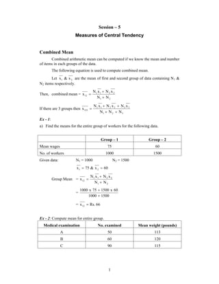
a) Find the means for the entire group of workers for the following data.
Group – 1 Group – 2
Mean wages 75 60
No. of workers 1000 1500
Given data: N1 = 1000 N2 = 1500
x 75 & x 60 1 2  
Group Mean =
12 N N
1 2
x


=

1000 1500
= x Rs. 66 12 
Ex - 2: Compute mean for entire group.
Medical examination No. examined Mean weight (pounds)
A 50 113
B 60 120
C 90 115

2.  
N x N x N x
 
(50 x 113 60 x120 90 x 115)
2
Combined mean (grouped mean weight)
1 1 2 2 3 3
N N N
 
1 2 3

x123  
(50 60 90)

x Mean weight 116 pounds 123  
Merits of Arithmetic Mean
1. It is simple and easy to compute.
2. It is rigidly defined.
3. It can be used for further calculation.
4. It is based on all observations in the series.
5. It helps for direct comparison.
6. It is more stable measure of central tendency (ideal average).
Limitations / Demerits of Mean
1. It is unduly affected by extreme items.
2. It is sometimes un-realistic.
3. It may leads to confusion.
4. Suitable only for quantitative data (for variables).
5. It can not be located by graphical method or by observations.
Geometric Mean (GM)
The GM is nth root of product of quantities of the series. It is observed by
multiplying the values of items together and extracting the root of the product
corresponding to the number of items. Thus, square root of the products of two items
and cube root of the products of the three items are the Geometric Mean.
Usually, geometric mean is never larger than arithmetic mean. If there are
zero and negative number in the series. If there are zeros and negative numbers in the
series, the geometric means cannot be used logarithms can be used to find geometric
mean to reduce large number and to save time.
In the field of business management various problems often arise relating to
average percentage rate of change over a period of time. In such cases, the arithmetic
mean is not an appropriate average to employ, so, that we can use geometric mean in
such case. GM are highly useful in the construction of index numbers.
Geometric Mean (GM) = 1 2 n n x x x x ...........x x
When the number of items in the series is larger than 3, the process of
computing GM is difficult. To over come this, a logarithm of each size is obtained.

3. The log of all the value added up and divided by number of items. The antilog of
quotient obtained is the required GM.
    
  
log log ................ log log x
i
(GM) = Antilog 
3




 N
Anti log
n
i 1
1 2 n
Merits of GM
a. It is based on all the observations in the series.
b. It is rigidly defined.
c. It is best suited for averages and ratios.
d. It is less affected by extreme values.
e. It is useful for studying social and economics data.
Demerits of GM
a. It is not simple to understand.
b. It requires computational skill.
c. GM cannot be computed if any of item is zero or negative.
d. It has restricted application.
Ex - 1:
a. Find the GM of data 2, 4, 8
x1 = 2,
x2 = 4,
x3 = 8
n = 3
GM = 1 2 3 n x x x x x
GM = 3 2 x 4 x 8
GM = 3 64  4
GM = 4
b. Find GM of data 2, 4, 8 using logarithms.
Data: x1 = 2
x2 = 4
x3 = 8
N = 3

4. 4
x log x
2 0.301
4 0.602
8 0.903
logx = 1.806

 
log x
GM = Antilog 

N


1.806
GM = Antilog 

3
GM = Antilog (0.6020)
= 3.9997
GM  4
Ex - 2:
Compare the previous year the Over Head (OH) expenses which went up to
32% in year 2003, then increased by 40% in next year and 50% increase in the
following year. Calculate average increase in over head expenses.
Let 100% OH Expenses at base year
Year OH Expenses (x) log x
2002 Base year –
2003 132 2.126
2004 140 2.146
2005 150 2.176
 log x = 6.448

 
log x
GM = Antilog 
N


6.448
GM = Antilog 

3
GM = 141.03
GM for discrete series
GM for discrete series is given with usual notations as month:

5. 5

 
log xi
GM = Antilog 

 N
i 1
Ex - 3:
Consider following time series for monthly sales of ABC company for 4
months. Find average rate of change per monthly sales.
Month Sales
I 10000
II 8000
III 12000
IV 15000
Let Base year = 100% sales.
Solution:
Month Base year
Sales
(Rs)
Increase /
decrease
%ge
Conversion
(x)
log (x)
I 100% 10000 – – –
II – 20% 8000 80 80 1.903
III + 50% 12000 130 130 2.113
IV + 25% 15000 155 155 2.190
logx = 6.206


6.206
GM = Antilog 

3
= 117.13
Average sales = 117.13 – 100 = 14.46%
Ex - 4: Find GM for following data.
Marks
(x)
No. of students
(f)
log x f log x
130 3 2.113 6.339
135 4 2.130 8.52
140 6 2.146 12.876
145 6 2.161 12.996
150 3 2.176 6.528
f = N = 22  f log x =47.23

6. 6

 
f log x
GM = Antilog 

N


22
GM = Antilog 

47.23
GM = 140.212
Geometric Mean for continuous series
Steps:
1. Find mid value m and take log of m for each mid value.
2. Multiply log m with frequency ‘f’ of each class to get f log m and sum up to
obtain  f log m.
3. Divide  f log m by N and take antilog to get GM.
Ex: Find out GM for given data below
Yield of wheat
in
MT
No. of farms
frequency
(f)
Mid value
‘m’
log m f log m
1 – 10 3 5.5 0.740 2.220
11 – 20 16 15.5 1.190 19.040
21 – 30 26 25.5 1.406 36.556
31 – 40 31 35.5 1.550 48.050
41 – 50 16 45.5 1.658 26.528
51 – 60 8 55.5 1.744 13.954
f = N = 100  f log m = 146.348

 
f logm
GM = Antilog 

N


146.348
GM = Antilog 
100
GM = 29.07
Harmonic Mean
It is the total number of items of a value divided by the sum of reciprocal of
values of variable. It is a specified average which solves problems involving
variables expressed in within ‘Time rates’ that vary according to time.

7. Ex: Speed in km/hr, min/day, price/unit.
Harmonic Mean (HM) is suitable only when time factor is variable and the act being
performed remains constant.
7
HM =
N

1
x
Merits of Harmonic Mean
1. It is based on all observations.
2. It is rigidly defined.
3. It is suitable in case of series having wide dispersion.
4. It is suitable for further mathematical treatment.
Demerits of Harmonic Mean
1. It is not easy to compute.
2. Cannot used when one of the item is zero.
3. It cannot represent distribution.
Ex:
1. The daily income of 05 families in a very rural village are given below. Compute
HM.
Family Income (x) Reciprocal (1/x)
1 85 0.0117
2 90 0.01111
3 70 0.0142
4 50 0.02
5 60 0.016
 1 = 0.0738
x
HM =
x
N

1
5
=
0.0738
= 67.72
HM = 67.72

8. 2. A man travel by a car for 3 days he covered 480 km each day. On the first day he
drives for 10 hrs at the rate of 48 KMPH, on the second day for 12 hrs at the rate
of 40 KMPH, and on the 3rd day for 15 hrs @ 32 KMPH. Compute HM and
weighted mean and compare them.
Harmonic Mean
x x
8
1
48 0.0208
40 0.025
32 0.0312
 1 = 0.0770
x
Data:
10 hrs @ 48 KMPH
12 hrs @ 40 KMPH
15 hrs @ 32 KMPH
HM =
x
N

1
3
=
0.0770
HM = 38.91
Weighted Mean
w x wx
10 48 480
12 40 480
15 32 480
w = 37 wx = 1440
Weighted Mean =
wx
w
x



=
1440
37
x  38.91
Both the same HM and WM are same.

9. 9
3. Find HM for the following data.


m
Class (CI) Frequency (f) Mid point (m) Reciprocal 

1


m
f 

1
0 – 10 5 5 0.2 1
10 – 20 15 15 0.0666 0.999
20 – 30 25 25 0.04 1
30 – 40 8 35 0.0285 0.228
40 – 50 7 45 0.0222 0.1554
f = 60


m
 f 

1
= 3.3824
HM =


 

1
m
f
N
60
=
3.3824
HM = 17.73
Relationship between Mean, Geometric Mean and Harmonic Mean.
1. If all the items in a variable are the same, the arithmetic mean, harmonic mean and
Geometric mean are equal. i.e., x GM  HM.
2. If the size vary, mean will be greater than GM and GM will be greater than HM.
This is because of the property that geometric mean to give larger weight to
smaller item and of the HM to give largest weight to smallest item.
Hence, x GM  HM.
Median
Median is the value of that item in a series which divides the array into two
equal parts, one consisting of all the values less than it and other consisting of all the
values more than it. Median is a positional average. The number of items below it is
equal to the number. The number of items below it is equal to the number of items
above it. It occupies central position.
Thus, Median is defined as the mid value of the variants. If the values are
arranged in ascending or descending order of their magnitude, median is the middle
value of the number of variant is odd and average of two middle values if the number
of variants is even.
Ex: If 9 students are stand in the order of their heights; the 5th student from either side
shall be the one whose height will be Median height of the students group. Thus,
median of group is given by an equation.

10.  
N 1 th item = 
 
N 1 th item = 
N 1 th item, a separate column is to be prepared for cumulative
10

 
N 1
Median = 

2
Ex
1. Find the median for following data.
22 20 25 31 26 24 23
Arrange the given data in array form (either in ascending or descending order).
20 22 23 24 25 26 31

 
Median is given by 

2


7 1
2
8
Median = 4th item.
=
4
2. Find median for following data.
20 21 22 24 28 32

 
Median is given by 

2


6 1
2
Median = 3.5th item.
The item lies between 3rd and 4.
So, there are two values 22 and 24.
The median value will be the mean values of these two values.

 
22 24
Median = 

2
= 23
Discrete Series – Median
In discrete series, the values are (already) in the form of array and the
frequencies are 
recorded against each value. However, to determine the size of
 

median 
2
frequencies. The median size is first located with reference to the cumulative
frequency which covers the size first. Then, against that cumulative frequency, the
value will be located as median.

11. Ex: Find the median for the students’ marks.
Obtained in statistics
1
2
3
4 1 6
5 1 7
6 2 9
7 2 11
8 2 13
9 2 15
11
Marks (x)
No. of
students (f)
Cumulative
frequency
10 5 5
20 5 10
30 3 13
40 15 28
50 30 58
60 10 68
N = 68
Ex: In a class 15 students, 5 students were failed in a test. The marks of 10 students
who have passed were 9, 6, 7, 8, 9, 6, 5, 4, 7, 8. Find the Median marks of 15
students.
Marks No. of students (f) cf
0
5
f = 15
Median =
N1th
2
item
Me =
151
2
= 8th
Me 8th item covers in cf of 9. the marks against cf 9 is 6 and hence
Median = 6
Just above 34
is 58. Against
58 c.f. the
value is 50
which is
median value

12. 12
Continuous Series
The procedure is different to get median in continuous series. The class
intervals are already in the form of array and the frequency are recorded against each
class interval. For determining the size, we should take
th
2
n
item and median class
located accordingly with reference to the cumulative frequency, which covers the size
first. When the median class is located, the median value is to be interpolated using
formula given below.

 h
 N
C
Median = 

2
f

Where
0 1  
2


 where,  0 is left end point of N/2 class and l1is right end
point of previous class.
h = Class width, f = frequency of median clas
C = Cumulative frequency of class preceding the median class.
Ex: Find the median for following data. The class marks obtained by 50 students are
as follows.
CI Frequency (f) Cum.
frequency (cf)
10 – 15 6 6
15 – 20 18 24
20 – 25 9 33  N/2 class
25 – 30 10 43
30 – 35 4 47
35 – 40 3 50
f = N = 50
25
N  50

2
2
Cum. frequency just above 25 is 33 and hence, 20 – 25 is median class.
0 1  
2



20

20 20 
2
  20
h = 20 – 15 = 5

13. N 
 195
Cum. frequency just above 195 is 267.
13
f = 9
c = 24

 h
 N
C
Median = 

2
f

5
Median = 20 25 
24
9
=
5
9
20 
Median = 20.555
Ex: Find the median for following data.
Mid values (m) 115 125 135 145 155 165 175 185 195
Frequencies (f) 6 25 48 72 116 60 38 22 3
The interval of mid-values of CI and magnitudes of class intervals are same
i.e. 10. So, half of 10 is deducted from and added to mid-values will give us the lower
and upper limits. Thus, classes are.
115 – 5 = 110 (lower limit)
115 – 5 = 120 (upper limit) similarly for all mid values we can get CI.
CI Frequency (f) Cum.
frequency (cf)
110 – 120 6 6
120 – 130 25 31
130 – 140 48 79
140 – 150 72 151
150 – 160 116 267 N/2 class
160 – 170 60 327
170 – 180 38 365
180 – 190 22 387
190 – 200 3 390
f = N = 390
390
2
2

14. 14
Median class = 150 – 160
 =
150  150
2
= 150
h = 116
N/2 = 195
C = 151
h = 10

 h
 N
C
Median = 

2
f

10
Median = 150 195 
151
116
Median = 153.8
Merits of Median
a. It is simple, easy to compute and understand.
b. It’s value is not affected by extreme variables.
c. It is capable for further algebraic treatment.
d. It can be determined by inspection for arrayed data.
e. It can be found graphically also.
f. It indicates the value of middle item.
Demerits of Median
a. It may not be representative value as it ignores extreme values.
b. It can’t be determined precisely when its size falls between the two values.
c. It is not useful in cases where large weights are to be given to extreme values.