The document compares the low field electron transport properties in compounds of groups III-V semiconductors by solving the Boltzmann equation using an iterative technique. It calculates the temperature and doping dependencies of electron mobility in InP, InAs, GaP and GaAs. The electron mobility decreases with increasing temperature from 100K to 500K for each material due to increased electron-phonon scattering. Electron mobility also increases significantly with higher doping concentration at low temperatures. The iterative results show good agreement with other calculations and experiments. Electron mobility is highest in InAs and lowest in GaP at 300K, due to differences in their effective masses.

1. International Journal of Engineering Inventions
ISSN: 2278-7461, www.ijeijournal.com
Volume 1, Issue 2 (September 2012) PP: 56-61
Comparison of Low Field Electron Transport Properties in
Compounds of groups III-V Semiconductors by Solving
Boltzmann Equation Using Iteration Model
H. Arabshahi1, A. Pashaei2 and M. H .Tayarani3
1
Physics Department, Payame Noor University, P. O. Box 19395-4697, Tehran, Iran
23
Physics Department, Higher Education Khayyam, Mashhad, Iran
Abstract––Temperature and doping dependencies of electron mobility in InP, InAs,GaP and GaAs structures have been
calculated using an iterative technique. The following scattering mechanisms, i.e, impurity, polar optical phonon,
acoustic phonon and piezoelectric are included in the calculation. The electron mobility decreases monotonically as the
temperature increase from 100 K to 500 K for each material which is depended to their band structures characteristics.
The low temperature value of electron mobility increases significantly with increasing doping concentration. The
iterative results are in fair agreement with other recent calculations obtained using the relaxation-time approximation
and experimental methods.
Keywords–– Iterative technique; Ionized impurity scattering; Born approximation; electron mobility
I. INTRODUCTION
The problems of electron transport properties in semiconductors have been extensively investigated both
theoretically and experimentally for many years. Many numerical methods available in the literature (Monte Carlo method,
Iterative method, variation method, Relaxation time approximation, or Mattiessen's rule) have lead to approximate solutions
to the Boltzmann transport equation [1-2]. In this paper iterative method is used to calculate the electron mobility of InAs,
GaAs, InP and Gap. Because of high mobility InP has become an attractive material for electronic devices of superior
performance among the IIIphosphates semiconductors.Therefore study of the electron transport in group IIIphosphates is
necessary. GaP possesses an indirect band gap of 0.6 eV at room temperature whereas InP have a direct band gap about 1.8
eV, respectively. InP and InAs offer the prospect of mobility comparable to GaAs and are increasingly being developed for
the construction of optical switches and optoelectronic devices.
The low-field electron mobility is one of the most important parameters that determine the performance of a field-
effect transistor. The purpose of the present paper is to calculate electron mobility for various temperatures and ionized-
impurity concentrations. The formulation itself applies only to the central  valley conduction band. We have also consider
band nonparabolicity and the screening effects of free carriers on the scattering probabilities. All the relevant scattering
mechanisms, including polar optic phonons, deformation potential, piezoelectric, acoustic phonons, and ionized impurity
scattering. The Boltzmann equation is solved iteratively for our purpose, jointly incorporating the effects of all the scattering
mechanisms [3-4].This paper is organized as follows. Details of the iteration model , the electron scattering mechanism
which have been used and the electron mobility calculations are presented in section II and the results of iterative
calculations carried out on Inp,InAs,GaP,GaAs structures are interpreted in section III.
II. MODEL DETAIL
To calculate mobility, we have to solve the Boltzmann equation to get the modified probability distribution
function under the action of a steady electric field. Here we have adopted the iterative technique for solving the Boltzmann
transport equation. Under the action of a steady field, the Boltzmann equation for the distribution function can be written as
f eF f
 v. r f  . k f  ( ) coll (1)
t  t
Where (f / t ) coll represents the change of distribution function due to the electron scattering. In the steady-state and
under application of a uniform electric field the Boltzmann equation can be written as
eF f
. k f  ( ) coll (2)
 t
Consider electrons in an isotropic, non-parabolic conduction band whose equilibrium Fermi distribution function is f0(k) in
the absence of electric field. Note the equilibrium distribution f0(k) is isotropic in k space but is perturbed when an electric
field is applied. If the electric field is small, we can treat the change from the equilibrium distribution function as a
56

2. Comparison of Low Field Electron Transport Properties in Compounds of groups…
perturbation which is first order in the electric field. The distribution in the presence of a sufficiently small field can be
written quite generally as
f (k )  f 0 (k )  f1 (k ) cos  (3)
Where θ is the angle between k and F and f1(k) is an isotropic function of k, which is proportional to the magnitude of the
electric field. f(k) satisfies the Boltzmann equation 2 and it follows that:
eF  f0
 t i 
 1 i
 0 i 0
3

   cos  f  S  (1  f )  S f d k  f  S (1  f  )  S f   d k 
1 i
 0

i 0  
3
 (4)
In general there will be both elastic and inelastic scattering processes. For example impurity scattering is elastic and
acoustic and piezoelectric scattering are elastic to a good approximation at room temperature. However, polar and non-
polar optical phonon scattering are inelastic. Labeling the elastic and inelastic scattering rates with subscripts el and inel
respectively and recognizing that, for any process i, seli(k’, k) = seli(k, k’) equation 4 can be written as
 eF f 0
   f1cos [ Sinel (1  f 0 )  Sinel f 0 ] d 3k 

f1 (k )   k (5)
  (1  cos )Sel d 3k     [Sinel (1  f0 )  Sinel f0] d 3k 

Note the first term in the denominator is simply the momentum relaxation rate for elastic scattering. Equation 5 may be
solved iteratively by the relation
 eF f 0
   f1cos [n  1][Sinel (1  f 0 )  Sinel f 0 ] d 3k 

f1n (k )   k (6)
  (1  cos )Sel d 3k     [Sinel (1  f0 )  Sinel f0] d 3k 

Where f 1n (k) is the perturbation to the distribution function after the n-th iteration. It is interesting to note that if the initial
distribution is chosen to be the equilibrium distribution, for which f 1 (k) is equal to zero, we get the relaxation time
approximation result after the first iteration. We have found that convergence can normally be achieved after only a few
iterations for small electric fields. Once f 1 (k) has been evaluated to the required accuracy, it is possible to calculate
quantities such as the drift mobility  which is given in terms of spherical coordinates by

 (k / 1  2 F ) f1 d 3 k
3

  * 0
 (7)
3m F
k
2 3
f0d k
0
Here, we have calculated low field drift mobility in III-V structures using the iterative technique. In the following
sections electron-phonon and electron-impurity scattering mechanisms will be discussed.
Deformation potential scattering
The acoustic modes modulate the inter atomic spacing. Consequently, the position of the conduction and valence
band edges and the energy band gap will vary with position because of the sensitivity of the band structure to the lattice
spacing. The energy change of a band edge due to this mechanism is defined by a deformation potential and the resultant
scattering of carriers is called deformation potential scattering. The energy range involved in the case of scattering by
acoustic phonons is from zero to 2vk  , where v is the velocity of sound, since momentum conservation restricts the
change of phonon wave vector to between zero and 2k, where k is the electron wave vector. Typically, the average value of k
is of the order of 107 cm-1 and the velocity of sound in the medium is of the order of 10 5 cms-1. Hence, 2vk  ~ 1 meV,
which is small compared to the thermal energy at room temperature. Therefore, the deformation potential scattering by
acoustic modes can be considered as an elastic process except at very low temperature. The deformation potential scattering
rate with either phonon emission or absorption for an electron of energy E in a non-parabolic band is given by Fermi's
golden rule as [3,5]
2 D 2 ac (mt ml )1/ 2 K BT E (1  E )
*2 *
Rde 
 v 2  4 E (1  2E ) (8)
(1  E ) 2
 1 / 3(E ) 2 
Where Dac is the acoustic deformation potential,  is the material density and  is the non-parabolicity coefficient. The
formula clearly shows that the acoustic scattering increases with temperature
Piezoelectric scattering
The second type of electron scattering by acoustic modes occurs when the displacements of the atoms create an
electric field through the piezoelectric effect. The piezoelectric scattering rate for an electron of energy E in an isotropic,
parabolic band has been discussed by Ridley [4] .
57

3. Comparison of Low Field Electron Transport Properties in Compounds of groups…
The expression for the scattering rate of an electron in a non-parabolic band structure retaining only the important terms can
be written as [3,5]:
2
e 2 K B TK av m*
R PZ (k )   1 2 1  2 
2 2   s 2
 2
1     3 ( ) 
2 1 (9)
 
Where s is the relative dielectric constant of the material and Kav is the dimensionless so called average
electromechanical coupling constant.
Polar optical phonon scattering
The dipolar electric field arising from the opposite displacement of the negatively and positively charged atoms
provides a coupling between the electrons and the lattice which results in electron scattering. This type of scattering is called
polar optical phonon scattering and at room temperature is generally the most important scattering mechanism for electrons
in III-V .The scattering rate due to this process for an electron of energy E in an isotropic, non-parabolic band is [3-5]
 e2 2m*   1 1  1  2E 

RPO k  PO
  
8         E  (10)
 
FPO E , EN op , N op  1
Where E = E'±_wpo is the final state energy phonon absorption (upper case) and emission (lower case) and Nop is
the phonon occupation number and the upper and lower cases refer to absorption and emission, respectively. For small
electric fields, the phonon population will be very close to equilibrium so that the average number of phonons is given by the
Bose- Einstein distribution.
Impurity scattering
This scattering process arises as a result of the presence of impurities in a semiconductor. The substitution of an
impurity atom on a lattice site will perturb the periodic crystal potential and result in scattering of an electron. Since the mass
of the impurity greatly exceeds that of an electron and the impurity is bonded to neighboring atoms, this scattering is very
close to being elastic. Ionized impurity scattering is dominant at low temperatures because, as the thermal velocity of the
electrons decreases, the effect of long-range Coulombic interactions on their motion is increased. The electron scattering by
ionized impurity centers has been discussed by Brooks Herring [6] who included the modification of the Coulomb potential
due to free carrier screening. The screened Coulomb potential is written as
e2 exp(q0r ) (11)
V (r ) 
4  0 s r
Where s is the relative dielectric constant of the material and q0 is the inverse screening length, which under no
degenerate conditions is given by
ne2 (12)
q0 
2
 0 s K BT
Where n is the electron density. The scattering rate for an isotropic, nonparabolic band structure is given by [3,5]
Ni e4 (1  2E )  b  (13)
Rim  Ln(1  b) 
3/ 2  1 b
32 2m   s ( ( E ))  
* 2
8 m*  ( E ) (14)
b
 2q0
2
Where Ni is the impurity concentration.
III. RESULTS
We have performed a series of low-field electron mobility calculations for GaP, InP, GaAs and InAs materials.
Low-field motilities have been derived using iteration methode.The electron mobility is a function of temperature and
electron concentration .
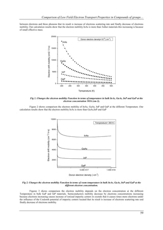
Figures 1 show the comparison the electron mobility depends on the Temperature at the different electron
concentration in bulk Gap,GaAs,InP and InAs materials. figures 1 show that electrons mobility at the definite temperature
300 k for the InAs semiconductors is gained about 8117cm2v-1s-1 and for GaAs, InP, Gap about 4883,4702,760 cm2v-1s-
1.also electrons mobility decrease quickly by temperature increasing from 200k to 500 k for all the different electron
concentrations because temperature increasing causes increase of phonons energy too. So it causes a strong interaction
58

4. Comparison of Low Field Electron Transport Properties in Compounds of groups…
between electrons and these phonons that its result is increase of electrons scattering rate and finally decrease of electrons
mobility. Our calculation results show that the electron mobility InAs is more than 3other materials this increasing is because
of small effective mass.
20000
16 -3
Donor electron density=10 ( cm )
InAs
Electron drift mobility (cm2 / V-s) 15000
10000
GaAs
5000 InP
GaP
0
200 250 300 350 400 450 500
Temperature (K)
Fig 1. Changes the electron mobility Function in terms of temperature in bulk InAs, GaAs, InP and GaP at the
electron concentration 1016 (cm-3).
Figure 2 shows comparison the electron mobility of InAs, GaAs, InP and GaP at the different Temperature .Our
calculation results show that the electron mobility InAs is more than GaAs,InP and GaP
10000
Temperature= 300 K
8000
Electron drift mobility (cm / V-s)
2
InAs
6000
4000 GaAs
InP
2000
GaP
5.00E+017 1.00E+018
-3
Donor electron density ( cm )
Fig 2. Changes the electron mobility Function in terms of room temperature in bulk InAs, GaAs, InP and GaP at the
different electron concentration.
Figures 3 shows comparison the electron mobility depends on the electron concentration at the different
Temperature in bulk GaP and InP materials. Semiconductors mobility decrease by electrons concentrations increasing
because electrons increasing causes increase of ionized impurity centers in crystals that it causes times more electrons under
the influence of the Coulomb potential of impurity centers located that its result is increase of electrons scattering rate and
finally decrease of electrons mobility
59

5. Comparison of Low Field Electron Transport Properties in Compounds of groups…
GaP:T=200 K
4000 GaP:T=300 K
InP:T=200 K
InP:T=300 K
Electron drift mobility (cm / V-s)
3000
2
2000
1000
5.00E+017 1.00E+018
Temperature (K)
Fig 3. Changes the electron mobility Function in terms of electron concentration in bulk InP and GaP at the different
Temperature
20000
16 -3
InAs:Ionized impurity densiy =10 [cm ]
17 -3
InAs:Ionized impurity densiy =10 [cm ]
16 -3
GaAs:Ionized impurity densiy =10 [cm ]
17 -3
GaAs:Ionized impurity densiy =10 [cm ]
Electron drift mobility (cm / V-s)
15000
2
10000
5000
200 250 300 350 400
Temperature (K)
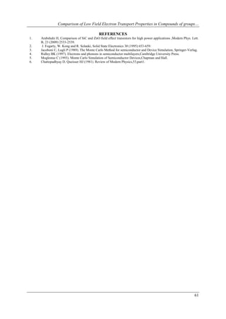
Fig 4. Changes the electron mobility Function in terms of temperature in bulk GaAs and InAs at the different electron
concentration.
Figures 4 shows comparison the electron mobility depends on temperature at the different electron concentration in bulk
InAs and GaAs materials. .Our calculation results show that the electron mobility InAs is more than GaAS
IV. CONCLUSION
1. InAs semiconductor having high mobility of GaAs,GaP and InP because the effective mass is small compared
with all of them
2. The ionized impurity scattering in all the semiconductor InAs,GaAs,InP and GaP at all temperatures is an
important factor in reducing the mobility.
60

6. Comparison of Low Field Electron Transport Properties in Compounds of groups…
REFERENCES
1. Arabshahi H, Comparison of SiC and ZnO field effect transistors for high power applications ,Modern Phys. Lett.
B, 23 (2009) 2533-2539.
2. J. Fogarty, W. Kong and R. Solanki, Solid State Electronics 38 (1995) 653-659.
3. Jacoboni C, Lugli P (1989). The Monte Carlo Method for semiconductor and Device Simulation, Springer-Verlag.
4. Ridley BK (1997). Electrons and phonons in semiconductor multilayers,Cambridge University Press.
5. Moglestue C (1993). Monte Carlo Simulation of Semiconductor Devices,Chapman and Hall.
6. Chattopadhyay D, Queisser HJ (1981). Review of Modern Physics,53,part1.
61