This document discusses methods for interpolating rainfall data using modified inverse distance weighting (MIDW) techniques. It examines four general forms of the MIDW method where the effects of distance and elevation difference can take positive or negative weights. The authors apply genetic algorithms to optimize the MIDW interpolation equation regionally and compare integrated vs. separated dimensionless weighting approaches. Daily rainfall data from 49 stations in the Mashhad plain catchment area of Iran over 16 years is analyzed. The results show that accounting for elevation improves interpolation and that regional optimization of the MIDW method leads to better performance than local optimization.

1. International Journal of Engineering Inventions
ISSN: 2278-7461, www.ijeijournal.com
Volume 1, Issue 3 (September 2012) PP: 57-65
Extended Modified Inverse Distance Method for Interpolation
Rainfall
Nafise Seyyednezhad Golkhatmi1, Seyed Hosein Sanaeinejad2, Bijan Ghahraman3,
Hojat Rezaee Pazhand4
1
Graduate student of agricultural meteorology
2
Ferdowsi University of Mashhad,Water Engineering Group
3
Ferdowsi University of Mashhad,Water Engineering Group
4
Islamic Azad University,Mashhad Branch, Department of Civil
Abstract––Local Interpolation and regional analyzing of rainfall are one of the important issues of Water Resources and
Meteorology. There are several methods for this purpose. IDW is one of the classic methods for estimating precipitation.
This method of interpolation at each point gives a weight to the distance to the reference point. IDW method has been
modified in various ways in different research and new parameters such as elevation were added to it. This reform has
two modes. The First state is the ratio of elevation to distance and the second is the inverse of multiplying elevation and
distance. This paper has three objectives. First is generalizing the alignments of various elevation and distances in
MIDW. Second is dimensionless the weights (separately and integrated) according to relationship that is used. Third is
analyzing interpolation errors of daily rainfall regionally. Genetic algorithm is used to find optimal answers. Results
showed that optimal answers primarily is depending on the reverse effects of multiply of altitude and distance (55%) and
with a direct effect of altitude and inverse effect of distance (45%). It's then 71% of cases shows that integrated
dimensionless yields better result than separately ones. Impacts of elevation were established in all MIDW methods.
Results showed that this parameter should be used in interpolation of rainfall. Case study is a daily rainfall catchment of
Mashhad plain.
Keywords––Regionally interpolation, MIDW, Genetic algorithm, Mashhad.
I. INTRODUCTION
Local and areal estimations of rainfall are needed in those projects and researches that used point, areal and
regional data of hydrology and climatology, areal and regional water use and weather. Ordinary methods for estimating this
Phenomenon includes the Arithmetic mean, Thiessen, Rainfall gradient, Inverse Distance and Isohyetal curves (Horton,
1923, Singh and Birsoy, 1975, Johansson, 2000). Finite element method (Hutchinson and Walley, 1972), Kriging (Vasiliades
and Loukas, 2009), Fuzzy Kriging (Bondarabadi and Saghafian, 2007) and splines (Hutchinson, 1998), Neural Networks
(Rigol et al, 2001, Moghaddam and et al, 2011) as well as relatively new methods for the spatial estimating for this
phenomenon.It can be corrected by conventional methods and acceptable results are achieved. One of these is the Inverse
Distance (IDW) method that some researchers have done some changes in it and called it Modified Inverse Distance method
(MIDW) (Lo, 1992, Chang et al, 2005). Lo (1992) introduced MIDW such that the impact of elevation difference in the IDW
is considered as a factor. Therefore, the weight of each station is to be distance to the elevation ratio with k power. This
relation is suitable for mountainous areas. Chen and Liu (2012) applied IDW method for regional analysis of 46 rain gauge
stations located in Taiwan. They investigated the influence of stations radiuses neighborhood too. Radiuses of the desired
effect are 10 to 30 km and fluctuations in the power of the IDW 1.5 to 4 obtained. Monthly and annual precipitation data
were used in their research. Tomczak (1998) performed spatial interpolation of precipitation with IDW method. He studied
two parameters, the distance and spherical radius and optimized the parameters of function with cross-validation. Then he
attempted with the Jack- Knife to determine the sampling frequency skew, the standard error and confidence intervals for
each station. He concluded that this method can obtain satisfactory results with respect to these two points.
Chang et al. (2005) combined the IDW method by Fuzzy theory for interpolation the missing data. Genetic
Algorithm also was employed to optimize the fuzzy membership function parameters. Daily rainfall of six rain gauge
stations (located in a catchment area of 303 sq km in northern Taiwan) were used for this proposed. Their research
investigated the equation errors of interpolation at each station separately. Estimation errors of precipitation from this
method are generally reported less than Thiessen and arithmetic averages methods. Lu (1992) added ratio of distance to
elevation and Chang et al. (2005) added the inverse of these two parameters products into the IDW method. The regional
rainfall analysis is affected by the elevation. It has a negative influence in the adjacent water resources areas (Coastal and
Forest) and positive in the remote areas (mountainous region). It is possible that to Modify IDW method by changing places
of its parameters and their powers. We can put each one in numerator or denominator of IDW’s coefficients separately or
tougher. So we have four states that they are more general than Chang et al. and Lo modified methods. We follow three
goals in this research. First, we compare these four methods. The various MIDW methods approaches to optimize MIDW
interpolation equation locally (Moghaddam et al., 2011, Tomczak, 1998,Chen and Liu, 2012). Second goal is modifying the
IDW method for optimizing interpolation equation regionally in Mashhad basin area (regional interpolation). Third we
57

2. Extended Modified Inverse Distance Method for interpolation rainfall
compare two dimensionless weighted methods of MIDW coefficients. So we have eight separated models for regional
interpolation MIDW in general. Our case study is Mashhad basin in Iran.
II. MATERIALS AND METHODS
1.2 Study area and data
The study region is the catchment area of Mashhad plain with 9909.4 sq km in longitude 580 – 20´ and 600 - 8´East
and latitude 360 - 0´and 370 - 5´North in North East of Iran. Mashhad plain is a basin with irregular topography, the climate
is arid, semi arid and its north and south is surrounded by tow mountain ranges by the name of Hezar-Masjed and Binaloud,
Respectively Number of rain gauge stations in this basin and its adjacent are 49 (each one with a 16 year data 1993-2009).
These stations are run under the Iran Ministry of Energy. 71days of daily rainfall data is used. The geographical position and
characteristics of stations come in Figure (1) and Table (2) respectively. SQL Server 2008 and VB.NET 2010 used for
Descriptive Statistics.
Figure (1) - Catchment location Mashhad plain with rain gauge stations in and around
2.2 Methods of Modified Inverse Distance (MIDW)
Modified Inverse Distance methods are obtained by changing the conventional Inverse Distance (IDW) weight.
Distances between stations are used for weighted IDW. While other factors such as elevation are also an important influence
on rainfall and can be a weight in IDW. Operating arrangement of elevations and distances in the IDW is leads to a variety
d xi k
MIDW as follows. Lo (1992) introduced the MIDW according to equation (1). The weight of each station ( ( ) ) is
H xi
the ratio of distance ( d xi ) to the elevation difference ( H xi ). Indeed, impact of component difference is assumed to be
direct and impact of component elevation is reverse with identical power for both.
N
d
∑ H
( xi ) k .p i
p x  i 1
xi
, k0 (1)
N
d
∑ H ) k
( xi
i 1 xi
where p x is the Point Rainfall estimation, d xi is the distance between each station from the base station. Moreover, N is
the number of stations that used, k is the power’s parameter and H xi is difference elevation between base station and the
ith station.
Chang et al. (2005) have considered the inverse multiply of elevation and distances as a weight in MIDW. They
are considered different power for distance (m) and elevation (n) weight. Interpolation error equation in this method is
discussed locally (separately for each station). Formula (2) is the model of Chang et al. (2005).
58

3. Extended Modified Inverse Distance Method for interpolation rainfall
N
∑ xin * d xim )
h
Px = i =1
N
* Pi , m > 0, n > 0 (2)
∑ xin * d xim
h
i =1
Where: m and n are powers (parameters). h xi is the elevation difference between base station and ith’ ones. Other items are
the same as formula (1).
The defined model in this study is general pattern of equation (2). So that the distance and elevation difference are
allowed that have different alignment (positive or negative sign of m and n). So their effect is direct or inverse. In other
words, both appear in the numerator, or both in the denominator or one in the denominator and another in the numerator with
different power. Estimating the optimal m and n parameters are needed. Genetic algorithm is suitable for this purpose.
3.2 Genetic Algorithm
Genetic algorithm is a probabilistic search method that surrounds a natural biological process of evolution will
follow. This method is based on the Darwinian theory of evolution and Encodes the potential solutions to a problem to
chromosomes in a simple format. Then implement the combination operators with a random population of individuals (each
one in the form of chromosome), (Kia, 2009). Genetic algorithm can produce many generations. The initial population is
generated randomly in the desired interval. New set of approximations in each generation with the best member selection
process based on their fitness in the problem domain and the multiplication of the operators are made from natural genetics.
This process will ultimately lead to the evolution of population members that have better adaptation of the original members
of the original parents in their environment.
Members of the population or in other words, the current approximation of the optimal solution encodes as string
by sequence into the chromosome with the variables of the problem. Objective function, provides an index to select the
appropriate pair and mating chromosomes in the population. After the initial generation, the next generation is produced
using genetic operations such as elitism, mating (crossover) and mutation. Each member shall be entitled to represent the
value of its compatibility (with the objective function). Members who have a higher consistency than others will have a
higher chance to select and move to the next generation and vice versa (elitism). Mating genetic operator combines the genes
of chromosomes together, but does not necessarily act on all the strings of population. The contrary, it is done with
probability p. Mutation operator is performed with a random selection of chromosomes and random selection of one or more
genes and substituting its contradictory. The mutation also will act with prior probability (pm). Thus continues the cycle of
next generations. The end of the genetic algorithm process is achieving optimal solutions (Shabani Nia and Saeed Nia, 2009,
Kia, 2009). Genetic algorithm is used for estimation and to optimize the variables of interpolation equations and due to time
savings. MIDW method is interpolating method with two m and n parameters where m is power of distance factor and n is
power of the elevation factor. Two parameters (m and n) are generated randomly, and the error function is optimized with
the repeat the algorithm and produced better m and n in each generation. The objective function in MIDW is minimizing the
regional mean absolute errors (MAE), (Equation 9). That is the mean of all local absolute errors. Chromosomes are the two
parameters; m and n (20 chromosomes in each generation) and are generated randomly according to GA operators. Two
adaptable chromosomes in each generation are transferred directly to the next generation (elitism). Genetic algorithm has
been programmed in MATLAB 7.8.0 (R2009). It is necessary to preprocessing data before analyzing that it is explained in
Next section.
2.4 Screening and normalization data and dimensionless weights
Available data are often mixed with error. These errors are the basis of false recorded, incorrect transfer, system
failures, etc. Data must first be screened. If data are not properly screened the elevation difference and distance should be
normalized to the same scale in MIDW (Chang et al, 2006, Hebert and Keenleyside,1995). Equation (3) and (4) is used for
normalization. This conversion causes the Elevation difference and distance should be between 1 and 10.
d d min
d′ 1 + 9 * (
= ) (3)
d max d min
h h min
h′ 1 + 9 * (
= ) (4)
h max - h min
- The dimensionless weights obtain with two methods: integration (Equation 5) and separation (Equation 6). If m and n are
assumed to be in the denominator (m and n are both negative), then integration and separation methods are the same as
equation (5) and (6). Other arrangements can be made similarly.
- The integrated dimensionless: dimensionless factor is the sum of multiplication of the distance and Elevation, (equation 5),
(Chang et al, 2005).
59

4. Extended Modified Inverse Distance Method for interpolation rainfall
N 1
∑ m
, m > 0, n > 0 )5(
i =1 d pi * hn
pi
- The separation dimensionless: dimensionless factor is the multiplication sum of the distance and elevation, (equation 6),
(Chang et al, 2005).
N 1 n 1
∑ m
* ∑ n , m > 0, n > 0 )6(
i =1 d pi i =1 h pi
The final equations for MIDW are (7) and (8) in the case that m and n are in the denominator. The rest of the functions for
other states of m and n are similar.
1 1
m
* n
N N dP hP
Px = ∑WdPi ,hP * Pi = ∑N i i
* Pi , m > 0, n > 0 )7(
i 1 1
i =1 i =1
∑m * n
i =1 d P hP
i i
1 1
* n
N N dm
Pi hP
Px = ∑WdPi ,hP * Pi = ∑ N i
N 1
* Pi , m > 0, n > 0 )8(
i 1
i =1 i =1
∑ m *∑ n
i =1 d P i =1 h P
i i
Eight error functions occur according to the descriptions, elevation and distance alignment and type of dimensionless. One of
them is in equation (9), (e.g. inverse of the distance and positive impact of the Elevation in separation dimensionless
method).
N
∑ n * d xim .Pi
h xi
N N i =1
i≠ j
E= ∑i = ∑ i*
e p N N
, m > 0, n > 0 )9(
i =1 i =1
∑ n * ∑ xim
h xi d
i =1 i =1
i≠ j i≠ j
Where p x is the observed rainfall in the ith station, and the second term is estimated rainfall in that station. Other items are
the same as formula (1). The error function is regulated similarly to the other seven cases (9).
III. RESULTS AND DISCUSSION
Data analysis in this article is 49 stations daily precipitation of Mashhad plain catchment for 16 years. A sample
size of 71 days is randomly selected and analyzed. Initially suspected precipitation was determined and The data were
screened. Then data normalized using equation (3) and (4). Analysis based on these normalized data. The purpose of this
study is to optimize the interpolation function (MIDW) and considering four general substitution of distance and Elevation to
explore the direct or reverse impact on daily rainfall interpolation multiple alignment is obtained by changing the sign of m
and n (power distance and Elevation). m and n parameters are optimized with genetic algorithm. Dimensionless of weights
of MIDW equation is done with equation (5) and (6). So in order to determine the best interpolation formula was studied in
eight states. Four states (substitution distance and elevation) were compared to determine the best relationship MIDW and
two for the best dimensionless. Genetic algorithm because of high-volume of calculations was used to determine the optimal
parameters. The work is as follows.
- Determine the number of required
First, the necessary population was determined to achieve the optimal response. Ten days were randomly selected
and was tested with 5 to 100 generations were divided into steps. Number of generations required to achieve the optimal
response was generally less than 50 numbers. Most of the generations required to achieve stability in the optimal solution
was obtained with 90 generations. Number of generations was chosen to ensure 100 more. Maximum and minimum errors
were calculated separately for each of the eight states MIDW. Errors in the eight-state amplitude were less than 10 mm. The
lowest error in each method with its parameters was chosen as the optimal errors and the desired parameters.
60

5. Extended Modified Inverse Distance Method for interpolation rainfall
- Effect of various alignments and types of Dimensionless
Alignment of distance and elevation were done in MIDW and algorithm were implemented and compared for each
state. This was compared with the index negative and positive coefficient for power distance (m) and elevation difference
(n). Moreover, dimensionless of weights were done in two ways (equations 5 and 6). Results are shown in Table (2).
Dimensionless indicated that all four alignments may not be necessary. Different states of the following below:
Dimensionless with equation (5):
Role of the distance and Elevation is reversed in 54% of cases (method of Chang et al.),31% of cases the influence
of distance is reversed and the influence of elevation is direct. For 10% of cases the influence of elevation is reversed and the
influence of distance is direct(Lu method) and in 6% of cases the influence of distance and elevation is direct. There are
necessary four alignments with different importance in this dimensionless. Distance and elevation never had zero impact on
the optimal solution.
B – Dimensionless with equation (6)
The influence of elevation difference and distance in 55% of cases was reversed (Chang et al method, 2005) and in
45% of other states influence of distance was reverse and influence of elevation was direct (of Lo, 1992), (Table 2) . Other
alignments in any case no optimal solution. Not eliminate the impact of distance in any equation. However, in the separation
dimensionless, In that case, the influence of elevation is director inverse and influence of direct or inverse, m was zero in
four cases. The following comparison of two methods showed that 87% of cases, equation (5) (the integration of weight and
Elevation) has the optimal solution and separation dimensionless state 13% of the cases has the optimal solution. Regional
best interpolation error equation with equation (9) is the calculated and regional average error is shown in Table (4(.Analysis
of error of regional interpolation equation for each day shows that lowest and highest errors are 1.3 and 8.2 mm respectively
(Table 4). Regional daily mean and standard deviation of errors (71 Days) are respectively 4 and 1.58 with a coefficient of
variation 39.5%. These results indicate that the accuracy of the interpolation equation is relatively good.
- Analyzing the range of m and n for 8 states of regional interpolation equations
Changes of m and n were evaluated for each eight methods. Results showed that changes of range for each
alignment of elevation and distance and each method of dimensionless are different (Table 3). If the influence of distance
and elevation is inversely (In both dimensionless methods) interval of m and n is [0, 16]. If the effect of distance to be
reversed and the effect of elevation be directed, m is between 1.14 to 15.98 and n between 2.09 to 15.98. When the effect of
elevation to be reversed and the effect of distance is directed (In both dimensionless methods), n changes from 0 to 4 and
changes m depends to the dimensionless method. So that changes due to the integrated dimensionless between 2.9 to 16 and
for the separation dimensionless between 0 and 3.07. More detail is shown in Table (3).
IV. CONCLUSION
The MIDW Interpolation method is used for precipitation. This method adds the elevation as a weight in IDW
equations. So far, two forms of MIDW were discussed. The first form is based on the distance to the elevation ratio (with
power constant k), and the second is based on the inverse of the distance and elevation with various m and n power. This
study extends the MIDW to its general form by considering eight weights which included the two previous forms. It includes
four forms of different alignment of distance and elevation and two methods of weights dimensionless (separation and
integrated). m and n present the power of distance and elevation in the models. Genetic algorithm was used to optimize the
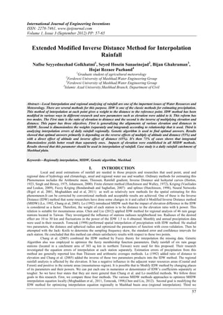
interpolation equation parameters of MIDW. Daily rainfall data for 49 stations of the Mashhad plain catchment was used in
this study. The results showed that the contribution of the integrated weights dimensionless is 87% and separate
dimensionless is 13% in optimization of different alignment of elevation and distance. Moreover, it is not necessary to
considerate all four types of alignment of elevation and distance for the studied areas. The results indicate that in the
separated method the role of the distance and elevation in 54% of cases are inverses (Equation 2). However, in 31% of cases,
the roles of distance is reverse and the role of elevation is direct, 10% of cases, the role of distance is direct and the role of
elevation is inverse (Equation 1), and 6% of cases, role of elevation and distance is direct. But in separated dimensionless,
the role of distance and elevation are reversed in 55% of cases, 45% of cases, the role of distance is direct and the role of
elevation is reversed. Two other alignments don’t have good answers in separated dimensionless and these equations were
excluded from MIDW. So to determine the best regional interpolation function, should not be limited to a specific alignment.
The study of six cases MIDW provides the possibility to achieve optimal solutions. A certain range cannot be considered for
parameters m and n, since large swings are observed in their intervals for eight states of MIDW. The average error and
standard deviation of the regional daily rainfall are 1.58 and 4 with coefficient of variation 39.5% respectively. The results
show that the accuracy of the interpolation equation is relatively good. The survey results showed using the MIDW method
with six different alignment of distance and elevation with two dimensionless in effective to achieve the optimal results.
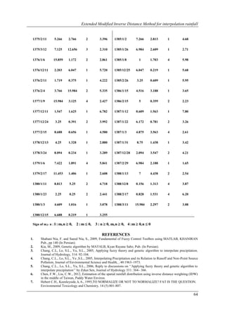
Table 1 - Characteristics Geographic stations in and around Mashhad catchment
Long. Lat. Long. Lat.
name elevation name elevation
(North) (west) (North) (west)
Dizbad Olya 1880 705752 3997566 Jong 1700 731149 4073827
Tabarokabad 1510 652515 4117177 Abghade Ferizi 1380 685763 4044656
61

6. Extended Modified Inverse Distance Method for interpolation rainfall
Heyhey 1330 636830 4105749 Goshe Bala 1580 728529 4066718
Eish Abade 1346 664428 4018975 All 1475 738067 4067314
Bar-Erie 1560 652778 4036255 Chenaran 1170 689618 4057478
Marusk 1495 638479 4043758 Moghan 1780 714164 4001945
Yengeje(Abshar) 1680 612457 4076877 Jaghargh 1420 708429 4021113
Cheshme Ali 1540 684471 4004990 Sharif Abad 1455 725852 3989818
Saghibaik 1510 626453 4064663 Talghor 1540 710308 4078053
Farhad Gerd 1500 746352 3961364 Ghadirabad 1175 676396 4074984
Golmakan 1400 693844 4040097 Chakane Olya 1780 631555 4078712
DahaneAkhlomad 1460 674033 4051676 Hesar Dehbar 1220 715841 4020953
Fariman 1395 760631 3955446 Hendel Abad 1210 768676 4035400
Radkan 1210 679342 4075224 Kalate Menar 990 791909 3981966
Dolatabad 1510 694409 4035379 Mayamei 1030 780656 4015387
Sadetorogh 1240 729639 4006280 Bazengan 1020 808510 4022543
Zoshk 1880 697502 4024363 Bahmanjan Olya 1340 675941 4086234
EdareMashhad 990 731039 4021956 Chahchahe 479 797692 4060098
Sar asiyabe
1270 709820 4031347 Gharetikan 520 784601 4079834
Shandiz
Androkh 1200 738131 4051588 Darband Kalat 970 742634 4098004
Sade karde 1300 738455 4056330 Archangan 745 731086 4110734
Mareshk 1870 727140 4077931 Hatamghale 490 709790 4132161
Olang Asadi 900 752266 4015822 Kabkan 1435 669345 4124444
Bande Saroj 1310 713617 4067555 LayenNow 876 721485 4112761
Bolghor 1920 731891 4081022
Table 2 - Effect of alignment of elevation and distance in MIDW with dimensionless weights
Separated (equation6) Integrated (equation 5)
percent alignment percent alignment
55.0% Elevation and distance is inverse 54.0% Elevation and distance is inverse
0.0% Elevation is direct and distance 31.0% Elevation is direct and distance
is inverse is inverse
0.0% Elevation and distance is direct 6.0% Elevation and distance is direct‫ا‬
45.0% Elevation is inverse and 10.0% Elevation is inverse and
distance is direct distance is direct
62

7. Extended Modified Inverse Distance Method for interpolation rainfall
Table (3) – Range of m and n in different MIDW methods
Separated (equation 6) Integrated (equation 5)
1.04 ≤ n ≤15.98 Elevation and 0.21 ≤ n ≤15.98 Elevation and 1
distance is inverse distance is inverse
0 ≤ m ≤13.78 1.14 ≤ m ≤15.98
- Elevation is direct 0.25 ≤ n ≤15.98 Elevation is direct 2
and distance is inverse and distance is inverse
2.09 ≤ m ≤15.98
- Elevation and 8.06 ≤ n ≤15.98 Elevation and 3
distance is direct distance is direct
1.59 ≤ m ≤15.98
1.15 ≤ n ≤3.15 Elevation is inverse 0.04 ≤ n ≤3.56 Elevation is inverse 4
and distance is direct and distance is direct
0 ≤ m ≤3.07 2.98 ≤ m ≤15.98
Table (4) - regional rainfall average absolute error Interpolation
Date (in sign Mean sign Mean
shamsi) m n m&n errors date m n m&n errors
1372/1/15 1.313 1.297 1 4.219 1380/2/1 3.359 1.75 1 3.50
1372/1/7 1.188 1.344 1 7.009 1380/2/11 5.422 1.047 2 3.94
1372/12/11 4.656 2.156 1 2.149 1380/2/23 4.797 0.5 2 6.40
1372/12/21 5.719 3.094 1 5.309 1381/1/25 14.266 2.969 2 4.08
1373/1/2 4.844 15.984 3 2.938 1381/1/29 14.984 10.359 1 4.43
1373/1/29 15.984 0.797 4 3.098 1381/12/22 3.953 15.984 2 2.99
1373/12/27 9 2.313 1 6.479 1381/2/19 3.938 0.531 1 6.70
1373/2/5 9.656 7.563 2 2.540 1381/3/4 4.484 0.406 1 3.27
1374/1/13 1.594 15.984 3 2.140 1382/1/1 2.734 1.625 2 4.69
1374/1/22 11.063 2.469 1 3.194 1382/1/17 8.266 0.047 4 4.63
1374/12/13 11.328 3.5 1 6.206 1382/12/25 2.281 0.844 1 5.29
1374/12/18 4.656 8.063 3 6.579 1382/2/9 6.5 3 2 3.82
1374/12/24 15.984 6.813 1 3.979 1383/1/6 13.109 1.453 1 4.59
1374/2/31 4.203 1.969 1 1.864 1383/12/24 8.219 0.813 1 4.62
1375/1/11 14.219 0.453 2 2.575 1383/2/21 5.25 3.313 1 2.54
1375/1/30 5.016 1.922 2 1.848 1384/1/19 3.484 0.922 1 8.18
1375/1/6 4.094 2.484 1 3.423 1384/12/10 15.875 8.422 1 3.14
1375/12/10 4.281 1.172 2 4.163 1385/1/11 2.438 1.781 1 1.28
63

8. Extended Modified Inverse Distance Method for interpolation rainfall
1375/2/11 5.266 2.766 2 3.396 1385/1/2 7.266 2.813 1 4.68
1375/3/12 7.125 12.656 3 2.310 1385/1/26 6.984 2.609 1 2.71
1376/1/6 15.859 1.172 2 2.861 1385/1/8 1 1.703 4 5.98
1376/12/11 2.203 6.047 1 5.720 1385/12/25 6.047 0.219 1 5.68
1376/2/11 1.719 0.375 1 4.222 1385/2/26 3.25 0.609 1 5.95
1376/2/4 3.766 15.984 2 5.335 1386/1/15 4.516 3.188 1 3.65
1377/1/9 15.984 3.125 4 2.427 1386/2/15 5 0.359 2 2.23
1377/12/11 1.547 1.625 1 6.782 1387/1/12 0.609 1.563 1 7.80
1377/12/24 3.25 0.391 2 3.992 1387/1/22 6.172 0.781 2 3.26
1377/2/15 8.688 0.656 1 4.580 1387/1/3 4.875 3.563 4 2.61
1378/12/13 4.25 1.328 1 2.880 1387/1/31 8.75 1.438 1 3.42
1378/3/24 8.094 0.234 1 3.289 1387/12/28 2.094 3.547 2 4.21
1379/1/6 7.422 1.891 4 5.841 1387/2/29 6.984 2.188 1 1.65
1379/2/17 11.453 1.406 1 2.608 1388/1/13 7 4.438 2 2.54
1380/1/11 8.813 5.25 2 4.718 1388/12/8 0.156 1.313 4 3.87
1380/1/23 2.25 0.25 2 2.441 1388/2/17 0.828 1.531 4 6.20
1380/1/3 4.609 1.016 1 3.078 1388/3/11 15.984 2.297 2 3.08
1380/12/15 6.688 0.219 1 3.255
Sign of m‫ و‬n : 1 : m, n  0, 2 : m  0, 3 : n  0, m, n  0, 4 :m  0, n  0
REFERENCES
1. Shabani Nia, F. and Saeed Nia, S., 2009, Fundamental of Fuzzy Control Toolbox using MATLAB, KHANIRAN
Pub., pp 140 (In Persian).
2. Kia, M., 2009, Genetic algorithm by MATALB, Kyan Rayane Sabz, Pub. (In Persian).
3. Chang, C.L, Lo, S.L., Yu, S.L., 2005, Applying fuzzy theory and genetic algorithm to interpolate precipitation.
Journal of Hydrology, 314: 92-104.
4. Chang, C.L., Lo, S.L., Yu ,S.L., 2005, Interpolating Precipitation and its Relation to Runoff and Non-Point Source
Pollution, Journal of Environmental Science and Health, , 40:1963–1973.
5. Chang, C.L., Lo, S.L., Yu, S.L., 2006, Reply to discussions on ‘‘Applying fuzzy theory and genetic algorithm to
interpolate precipitation’’ by Zekai Sen, Journal of Hydrology 331: 364– 366.
6. Chen, F.W., Liu, C.W., 2012, Estimation of the spatial rainfall distribution using inverse distance weighting (IDW)
in the middle of Taiwan, Paddy Water Environ.
7. Hebert C.H., Keenleyside, k.A., 1995,TO NORMALIZE OR NOT TO NORMALIZE? FAT IS THE QUESTION.
Environmental Toxicology and Chemistry, 14 (5):801-807.
64

9. Extended Modified Inverse Distance Method for interpolation rainfall
8. Dingman, S.L., 2002, PHYSICAL HYDROLOGY (SECOND EDITION). PRENTICE- HALL. Inc. 646 pp.
9. Ghazanfari M. M. S., Alizadeh, A., Mousavi B. S.M., Faridhosseini, A.R., Bannayan A. M. 2011, Comparison the
PERSIANN Model with the Interpolation Method to Estimate Daily Precipitation (A Case Study: North
Khorasan), Journal of Water and Soil. 25(1): 207-215.
10. Goovaerts, P., 2000, Geostatistical approaches for incorporating elevation into the spatial interpolation of rainfall.
Journalof Hydrology 228:113-29.
11. Horton, R.E., 1923, Monthly WEATHER REVIEW, ACCURACY OF AREAL RAINFALL ESTIMATES.
Consulting Hydraulic Engineer. 348-353.
12. Hutchinson, M.F., 1998, Interpolation of Rainfall Data with Thin Plate Smoothing Splines–Part II: Analysis of
Topographic Dependence, Journal of Geographic Information and Decision Analysis, 2(2): 152-167.
13. Hutchinson, P., Walley, W. J., 1972, CALCULATION OF AREAL RAINFALL USING FINITE ELEMENTS
TECHNIQUES WITH ALTITUDINAL CORRECTIONS. Bulletin of the International Association of
Hydrological Sciences, 259-272.
14. Johansson, B., 2000, Areal Precipitation and Temperature in the Swedish Mountains, An Evaluation from a
Hydrological Perspective. Nordic Hydrology, 31(3):207-228.
15. Rigol, J. P., Jarvis, C.H., Sturt, N., 2001, Artificial neural networks as a tool for spatial interpolation, int. j.
Geographical information science, 15(4): 323- 343.
16. Rahimi B.S., Saghafian, B., 2007, Estimating Spatial Distribution of Rainfall by Fuzzy Set Theory, Iran- Water
Resources Research, 3(2): 26-38.
17. LO, S. S., 1992, Glossary of Hydrology, W.R. Pub. ,PP 1794
18. Singh,V.P. and Birsoy,Y.,K.,1975, Comparison of the methods of estimating mean areal rainfall, Nordic
Hydrology 6(4): 222-241.
19. Tomczak, M., 1998, Spatial Interpolation and its Uncertainty Using Automated Anisotropic Inverse Distance
Weighting (IDW) - Cross-Validation/Jackknife Approach, Journal of Geographic Information and Decision
Analysis, 2(2): 18-30.
20. Vasiliades, L. and Loukas, A., 2009, PRECIPITATION SPATIAL INTERPOLATION METHODS
ASSESSMENT IN PINIOS RIVER BASIN, GREECE, Proceedings of the 11th international Conference on
Environmental Science and Technology,3-5.
65